Read KNMI observations using hydropandas
This notebook introduces how to use the hydropandas package to read, process and visualise KNMI data.
Martin & Onno - 2022
Notebook contents
Observation types
Get KNMI data
Get ObsCollections
Reference evaporation types
Spatial interpolation of evaporation
[1]:
import logging

import matplotlib.pyplot as plt
import numpy as np
import pandas as pd
from IPython.display import display
from scipy.interpolate import NearestNDInterpolator, RBFInterpolator
from tqdm import tqdm

import hydropandas as hpd
from hydropandas.io import knmi
[2]:
hpd.util.get_color_logger("INFO")
[2]:
<RootLogger root (INFO)>
Observation types
The hydropandas package has a function to read all kinds of KNMI observations. These are stored in an Obs object. There are three types of observations you can obtain from the KNMI:
EvaporationObs, for evaporation time seriesPrecipitationObs, for precipitation time seriesMeteoObs, for all the other meteorological time series
Get evaporation in [m/day] for KNMI station 344 (Rotterdam Airport).
[3]:
o = hpd.EvaporationObs.from_knmi(stn=344, start="2022")
display(o.head())
o.plot()
INFO:hydropandas.io.knmi.get_knmi_obs:get data from station 344 and variable EV24 from 2022-01-01 to None
hydropandas.EvaporationObs
| EV24_ROTTERDAM_344 | |
|---|---|
| x | 90061.930891 |
| y | 441636.854285 |
| location | |
| filename | |
| source | KNMI |
| unit | m |
| station | 344 |
| meteo_var | EV24 |
| EV24 | |
|---|---|
| YYYYMMDD | |
| 2022-01-01 01:00:00 | 0.0003 |
| 2022-01-02 01:00:00 | 0.0003 |
| 2022-01-03 01:00:00 | 0.0002 |
| 2022-01-04 01:00:00 | 0.0002 |
| 2022-01-05 01:00:00 | 0.0001 |
[3]:
<Axes: xlabel='YYYYMMDD'>

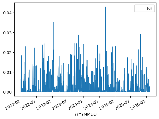
Get precipitation in [m/day] for KNMI station 344 (Rotterdam Airport).
[4]:
o = hpd.PrecipitationObs.from_knmi(stn=344, start="2022")
display(o.head())
o.plot()
INFO:hydropandas.io.knmi.get_knmi_obs:get data from station 344 and variable RH from 2022-01-01 to None
hydropandas.PrecipitationObs
| RH_ROTTERDAM_344 | |
|---|---|
| x | 90061.930891 |
| y | 441636.854285 |
| location | |
| filename | |
| source | KNMI |
| unit | m |
| station | 344 |
| meteo_var | RH |
| RH | |
|---|---|
| YYYYMMDD | |
| 2022-01-01 01:00:00 | 0.0000 |
| 2022-01-02 01:00:00 | 0.0002 |
| 2022-01-03 01:00:00 | 0.0064 |
| 2022-01-04 01:00:00 | 0.0000 |
| 2022-01-05 01:00:00 | 0.0008 |
[4]:
<Axes: xlabel='YYYYMMDD'>
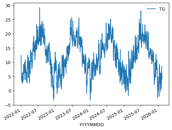
Get temperature in [°C] for KNMI station 344 (Rotterdam Airport).
[5]:
o = hpd.MeteoObs.from_knmi(stn=344, meteo_var="TG", start="2022")
display(o.head())
o.plot()
INFO:hydropandas.io.knmi.get_knmi_obs:get data from station 344 and variable TG from 2022-01-01 to None
hydropandas.MeteoObs
| TG_ROTTERDAM_344 | |
|---|---|
| x | 90061.930891 |
| y | 441636.854285 |
| location | |
| filename | |
| source | KNMI |
| unit | |
| station | 344 |
| meteo_var | TG |
| TG | |
|---|---|
| YYYYMMDD | |
| 2022-01-01 01:00:00 | 12.4 |
| 2022-01-02 01:00:00 | 12.1 |
| 2022-01-03 01:00:00 | 11.6 |
| 2022-01-04 01:00:00 | 9.7 |
| 2022-01-05 01:00:00 | 6.7 |
[5]:
<Axes: xlabel='YYYYMMDD'>
attributes
All PrecipitationObs, EvaporationObs and MeteoObs objects have the attributes:
name: meteo variable and station namex: x-coordinate in m RDy: y-coordinate in m RDstation: station numberunit: measurement unitmeta: dictionary with other metadata
[6]:
print(f"name: {o.name}")
print(f"x,y: {(o.x, o.y)}")
print(f"station: {o.station}")
print("unit", o.unit)
print("metadata:")
for key, item in o.meta.items():
    print(f"    {key}: {item}")
name: TG_ROTTERDAM_344
x,y: (np.float64(90061.9308913925), np.float64(441636.8542853093))
station: 344
unit
metadata:
    location: ROTTERDAM
    TG: Etmaalgemiddelde temperatuur (in graden Celsius) / Daily mean temperature in (degrees Celsius)
Get KNMI data
The from_knmi method can be used to obtain one type of measurements at one station. There are two ways to select the station.
with the station number
stnby specifying the
xycoordinates, the station nearest to this coordinates is used.
Below both methods are used to obtain precipitation measurements. Notice that they return the same data because station 344 is nearest to the given xy coordinates.
[7]:
o1 = hpd.PrecipitationObs.from_knmi(stn=344)
o2 = hpd.PrecipitationObs.from_knmi(xy=(90600, 442800))
o1.equals(o2)
INFO:hydropandas.io.knmi.get_knmi_obs:get data from station 344 and variable RH from None to None
INFO:hydropandas.io.knmi.get_knmi_obs:get KNMI data from station nearest to coordinates (90600, 442800) and meteovariable RH
[7]:
True
read options
The from_knmi method has other optional arguments:
stn: station number.start: the start date of the time series you want, default is 1st of January 2019.end: the end date of the time series you want, default is today.fill_missing_obs: option to fill missing values with values from the nearest KNMI station. If measurements are filled an extra column is added to the time series in which the station number is shown that was used to fill a particular missing value.interval: time interval of the time series, default is ‘daily’use_api: select the method to obtain the data, default is ‘True’raise_exception: option to raise an error when the requested time series is empty. ***
The 3 examples below give a brief summary of these options
[8]:
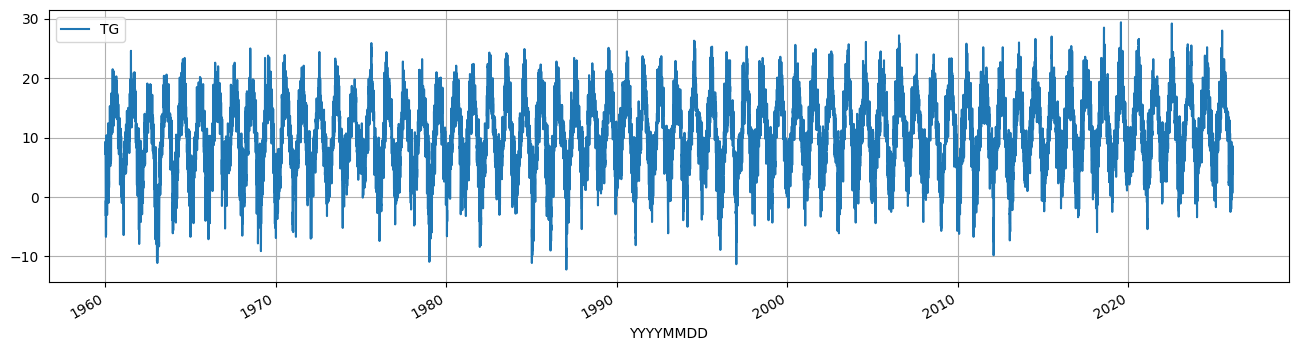
# example 1 get daily average temperature (TG) from 1900 till now
o_t = hpd.MeteoObs.from_knmi("TG", stn=344, start="1960")
o_t.plot(figsize=(16, 4), grid=True);
INFO:hydropandas.io.knmi.get_knmi_obs:get data from station 344 and variable TG from 1960-01-01 to None
[9]:
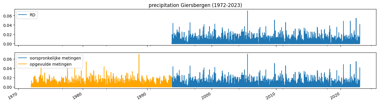
# example 2 get daily average precipitation from 1972 with and without filling missing measurements
f, axes = plt.subplots(figsize=(16, 6), nrows=2, sharex=True, sharey=True)

o_rd = hpd.PrecipitationObs.from_knmi(
    "RD", stn=892, start="1972", end="2023", fill_missing_obs=False
)
o_rd.plot(figsize=(16, 4), ax=axes[0])

o_rd_filled = hpd.PrecipitationObs.from_knmi(
    "RD", stn=892, start="1972", end="2023", fill_missing_obs=True
)

o_rd_filled.loc[o_rd_filled["station"] == "892", "RD"].plot(
    ax=axes[1], label="oorspronkelijke metingen"
)
o_rd_filled.loc[o_rd_filled["station"] != "892", "RD"].plot(
    ax=axes[1], color="orange", label="opgevulde metingen"
)
axes[0].set_title("precipitation Giersbergen (1972-2023)")
axes[1].legend();
INFO:hydropandas.io.knmi.get_knmi_obs:get data from station 892 and variable RD from 1972-01-01 to 2023-01-01
INFO:hydropandas.io.knmi.get_knmi_obs:get data from station 892 and variable RD from 1972-01-01 to 2023-01-01
INFO:hydropandas.io.knmi._add_missing_indices:station 892 has no measurements before 1993-11-01 09:00:00
INFO:hydropandas.io.knmi.fill_missing_measurements:Filled 7975 observations from station 827 TILBURG -> 892 GIERSBERGEN
[10]:
# see the station_opvulwaarde
display(o_rd_filled.head())
hydropandas.PrecipitationObs
| RD_GIERSBERGEN_892 | |
|---|---|
| x | 138500.0 |
| y | 407500.0 |
| location | |
| filename | |
| source | KNMI |
| unit | m |
| station | 892 |
| meteo_var | RD |
| RD | station | |
|---|---|---|
| 1972-01-01 09:00:00 | 0.0 | 827 |
| 1972-01-02 09:00:00 | 0.0 | 827 |
| 1972-01-03 09:00:00 | 0.0 | 827 |
| 1972-01-04 09:00:00 | 0.0 | 827 |
| 1972-01-05 09:00:00 | 0.0 | 827 |
[11]:
# example 3 get evaporation
logging.getLogger().getEffectiveLevel()
logging.getLogger().setLevel(logging.INFO)

o_ev = hpd.EvaporationObs.from_knmi(
    stn=344, start="1972", end="2023", fill_missing_obs=True
)
o_ev
INFO:hydropandas.io.knmi.get_knmi_obs:get data from station 344 and variable EV24 from 1972-01-01 to 2023-01-01
INFO:hydropandas.io.knmi._add_missing_indices:station 344 has no measurements before 1987-09-12 01:00:00
INFO:hydropandas.io.knmi.fill_missing_measurements:Filled 246 observations from station 210 VALKENBURG -> 344 ROTTERDAM
INFO:hydropandas.io.knmi.fill_missing_measurements:Filled 64 observations from station 348 CABAUW-MAST -> 344 ROTTERDAM
INFO:hydropandas.io.knmi.fill_missing_measurements:Filled 5499 observations from station 260 DE-BILT -> 344 ROTTERDAM
[11]:
hydropandas.EvaporationObs
| EV24_ROTTERDAM_344 | |
|---|---|
| x | 90061.930891 |
| y | 441636.854285 |
| location | |
| filename | |
| source | KNMI |
| unit | m |
| station | 344 |
| meteo_var | EV24 |
| EV24 | station | |
|---|---|---|
| 1972-01-01 01:00:00 | 0.0002 | 260 |
| 1972-01-02 01:00:00 | 0.0002 | 260 |
| 1972-01-03 01:00:00 | 0.0002 | 260 |
| 1972-01-04 01:00:00 | 0.0000 | 260 |
| 1972-01-05 01:00:00 | 0.0000 | 260 |
| ... | ... | ... |
| 2022-12-28 01:00:00 | 0.0003 | 344 |
| 2022-12-29 01:00:00 | 0.0001 | 344 |
| 2022-12-30 01:00:00 | 0.0002 | 344 |
| 2022-12-31 01:00:00 | 0.0001 | 344 |
| 2023-01-01 01:00:00 | 0.0001 | 344 |
18629 rows × 2 columns
Get ObsCollections
You can read multiple Observation objects at once using the hpd.read_knmi method. The observations are stored in an ObsCollection object. Below an example to obtain precipitation (RH) and evaporation (EV24) from the measurement stations Rotterdam (344) and De Bilt (260).
[12]:
oc = hpd.read_knmi(stns=[344, 260], meteo_vars=["RH", "EV24"])
oc
INFO:hydropandas.io.knmi.get_knmi_obs:get data from station 344 and variable RH from None to None
INFO:hydropandas.io.knmi.get_knmi_obs:get data from station 260 and variable RH from None to None
INFO:hydropandas.io.knmi.get_knmi_obs:get data from station 344 and variable EV24 from None to None
INFO:hydropandas.io.knmi.get_knmi_obs:get data from station 260 and variable EV24 from None to None
[12]:
| x | y | location | filename | source | unit | station | meteo_var | obs | |
|---|---|---|---|---|---|---|---|---|---|
| name | |||||||||
| RH_ROTTERDAM_344 | 90061.930891 | 441636.854285 | KNMI | m | 344 | RH | PrecipitationObs RH_ROTTERDAM_344 -----metadat... | ||
| RH_DE-BILT_260 | 140565.152506 | 456790.999119 | KNMI | m | 260 | RH | PrecipitationObs RH_DE-BILT_260 -----metadata-... | ||
| EV24_ROTTERDAM_344 | 90061.930891 | 441636.854285 | KNMI | m | 344 | EV24 | EvaporationObs EV24_ROTTERDAM_344 -----metadat... | ||
| EV24_DE-BILT_260 | 140565.152506 | 456790.999119 | KNMI | m | 260 | EV24 | EvaporationObs EV24_DE-BILT_260 -----metadata-... |
other options in the read_knmi function are:
specify
locationsas a dataframe with x, y coordinates (RD_new), the function will find the nearest KNMI station for every location.specify
xmidandymidwhich are 2 arrays corresponding to a structured grid to obtain the nearest KNMI station for every cell in the grid.
[13]:
locations = pd.DataFrame(index=["Rotterdam"], data={"x": 90600, "y": 442800})
display(locations)
hpd.read_knmi(locations=locations, meteo_vars=["RH"])
| x | y | |
|---|---|---|
| Rotterdam | 90600 | 442800 |
INFO:hydropandas.io.knmi.get_knmi_obs:get data from station 344 and variable RH from None to None
[13]:
| x | y | location | filename | source | unit | station | meteo_var | obs | |
|---|---|---|---|---|---|---|---|---|---|
| name | |||||||||
| RH_ROTTERDAM_344 | 90061.930891 | 441636.854285 | KNMI | m | 344 | RH | PrecipitationObs RH_ROTTERDAM_344 -----metadat... |
[14]:
hpd.read_knmi(xy=((90600, 442800),), meteo_vars=["RH"])
INFO:hydropandas.io.knmi.get_knmi_obs:get data from station 344 and variable RH from None to None
[14]:
| x | y | location | filename | source | unit | station | meteo_var | obs | |
|---|---|---|---|---|---|---|---|---|---|
| name | |||||||||
| RH_ROTTERDAM_344 | 90061.930891 | 441636.854285 | KNMI | m | 344 | RH | PrecipitationObs RH_ROTTERDAM_344 -----metadat... |
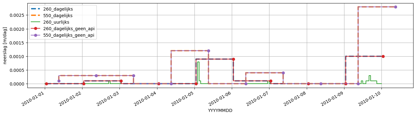
Precipitation
Using hydropandas 3 different precipitation products can be accessed:
Daily data from a meteorological station
Daily data from a neerslag (precipitation) station
Hourly data from a meteorological station
All three products can be obtained using the from_knmi method. Product 1 and 2 can also be accessed without the api.
By default data is used from a meteorological station. Specify meteo_var='RD' to access data from a neerslag (precipitation) station.
[15]:
start = "2010-1-1"
end = "2010-1-10"

# daily meteo station (default)
precip1 = hpd.PrecipitationObs.from_knmi(stn=260, start=start, end=end)
INFO:hydropandas.io.knmi.get_knmi_obs:get data from station 260 and variable RH from 2010-01-01 to 2010-01-10
[16]:
# daily neerslag station
precip2 = hpd.PrecipitationObs.from_knmi(meteo_var="RD", stn=550, start=start, end=end)
INFO:hydropandas.io.knmi.get_knmi_obs:get data from station 550 and variable RD from 2010-01-01 to 2010-01-10
[17]:
# hourly meteo station (only works with api)
precip3 = hpd.PrecipitationObs.from_knmi(
    stn=260,
    start=start,
    end=end,
    interval="hourly",
)
INFO:hydropandas.io.knmi.get_knmi_obs:get data from station 260 and variable RH from 2010-01-01 to 2010-01-10
[18]:
# daily meteo station without api
precip4 = hpd.PrecipitationObs.from_knmi(
    stn=260,
    start=start,
    end=end,
    use_api=False,
)
INFO:hydropandas.io.knmi.get_knmi_obs:get data from station 260 and variable RH from 2010-01-01 to 2010-01-10
[19]:
# daily neerslag station without api
precip5 = hpd.PrecipitationObs.from_knmi(
    meteo_var="RD",
    stn=550,
    start=start,
    end=end,
    use_api=False,
)
INFO:hydropandas.io.knmi.get_knmi_obs:get data from station 550 and variable RD from 2010-01-01 to 2010-01-10
Below are the differences between the precipitation estimates from different station types.
[20]:
fig, ax = plt.subplots(figsize=(16, 4))
precip1["RH"].plot(
    ax=ax,
    drawstyle="steps",
    ls="--",
    lw=3,
    label=str(precip1.station) + "_dagelijks",
)

precip2["RD"].plot(
    ax=ax,
    drawstyle="steps",
    ls="--",
    lw=3,
    label=str(precip2.station) + "_dagelijks",
)

precip3["RH"].plot(
    ax=ax,
    drawstyle="steps",
    label=str(precip3.station) + "_uurlijks",
)

precip4["RH"].plot(
    ax=ax,
    drawstyle="steps",
    marker="o",
    label=str(precip4.station) + "_dagelijks_geen_api",
)

precip5["RD"].plot(
    ax=ax,
    drawstyle="steps",
    marker="o",
    label=str(precip5.station) + "_dagelijks_geen_api",
)


ax.legend()
ax.grid()
ax.set_ylabel("neerslag [m/dag]");
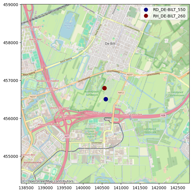
The locations of the stations can be plotted onto a map using the contextily package.
[21]:
import contextily as cx

oc = hpd.ObsCollection([precip1, precip2])

gdf = oc.to_gdf()

gdf = gdf.set_crs(28992)

gdf["name"] = gdf.index

ax = gdf.buffer(2000).plot(alpha=0, figsize=(8, 8))

gdf.plot("name", ax=ax, cmap="jet", legend=True, markersize=100)


cx.add_basemap(ax, crs=28992, source=cx.providers.OpenStreetMap.Mapnik)
Evaporation
KNMI provides the Makking reference evaporation (meteo_var EV24). Hydropandas provides a posssibility to calculate three different types of reference evaporation from data of KNMI meteo stations:
Penman
Hargreaves
Makkink (in the same way as KNMI)
These three types of reference evaporation are calculated the same way as described by Allen et al. 1990 and STOWA rapport. Be aware that the last report is written in Dutch and contains errors in the units.
The following variables from the KNMI are used for each reference evaporation type:
Penman: average (TG), minimum (TN) and maximum (TX) temperature, de global radiation (Q), de windspeed (FG) en de relative humidity (PG).
Hargreaves: average (TG), minimum (TN) and maximum (TX) temperature
Makkink: average temperature (TG) and global radiation (Q)
Comparison Makkink
Lets compare Hypdropandas Makkink verdamping evaporation with the EV24 Makkink verdamping of the KNMI. When Hydropandas Makkink evaporation is rounded (on 4 decimals), the estimate is the same as for the KNMI estimate.
[22]:
ev24 = hpd.EvaporationObs.from_knmi(
    stn=260, start="2022-1-1"
)  # et_type='EV24' by default
makk = hpd.EvaporationObs.from_knmi(meteo_var="makkink", stn=260, start="2022-1-1")
INFO:hydropandas.io.knmi.get_knmi_obs:get data from station 260 and variable EV24 from 2022-01-01 to None
INFO:hydropandas.io.knmi.get_knmi_obs:get data from station 260 and variable makkink from 2022-01-01 to None
[23]:
f, ax = plt.subplots(2, figsize=(11, 4))
ax[0].plot(ev24, label=ev24.name)
ax[0].plot(makk.round(4), label=makk.name)
ax[0].set_ylabel("E [m/d]")
ax[0].set_title("Makkink evaporation")
ax[0].legend()
ax[1].plot(ev24["EV24"] - makk["makkink"].round(4))
ax[1].set_title("Difference Makkink KNMI and Hydropandas")
f.tight_layout()

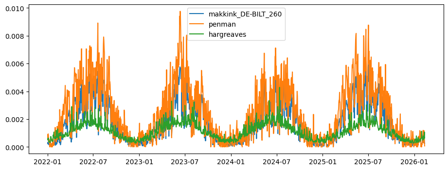
Comparison Penman, Makkink en Hargreaves
On average Penman gives a higher estimate for reference evaporation than Makkink (~0.55mm). This can be explained by the fact that Penman takes into account windspeed and Makkink ignores this proces. Hargreaves is a very simple way of estimation the evaporation, only taking into account temperature and extraterrestial radiation. Therefore it gives a lower estimate for the reference evporatoin compared to the two other methods (~-0.35mm wrt Makkink).
[24]:
penm = hpd.EvaporationObs.from_knmi(
    meteo_var="penman", stn=260, start="2022-1-1"
).squeeze()
harg = hpd.EvaporationObs.from_knmi(
    meteo_var="hargreaves", stn=260, start="2022-1-1"
).squeeze()
INFO:hydropandas.io.knmi.get_knmi_obs:get data from station 260 and variable penman from 2022-01-01 to None
INFO:hydropandas.io.knmi.get_knmi_obs:get data from station 260 and variable hargreaves from 2022-01-01 to None
[25]:
f, ax = plt.subplots(figsize=(11, 4))
ax.plot(makk, label=makk.name)
ax.plot(penm, label=penm.name)
ax.plot(harg, label=harg.name)
ax.legend()
[25]:
<matplotlib.legend.Legend at 0x7f75533130e0>
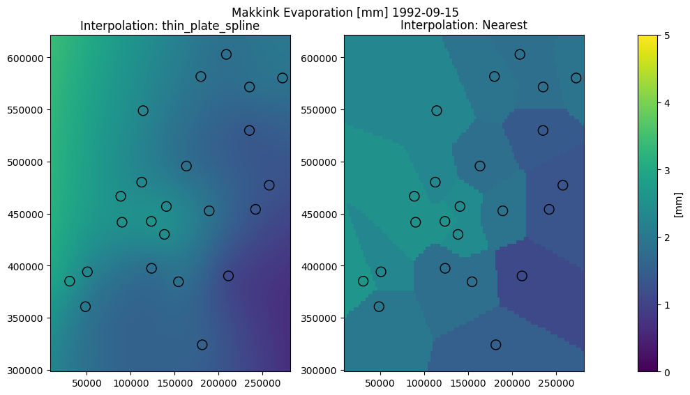
Spatial interpolate (Makkink) Evaporation?
Does interpolation matter? There are ways to interpolate evaporation datasets. However currently the nearest station is always used in HydroPandas’ methods. Does this give different results? First lets look spatially.
Get all stations where EV24 is measured
[26]:
stns = knmi.get_stations(meteo_var="EV24").sort_index()
Collect all EV24 data ever measured by KNMI
[27]:
tmin = "1950-01-01"
tmax = "2022-04-11"

# empty dataframe
df = pd.DataFrame(
    columns=stns.index
)  # index=pd.date_range(start=tmin, end=tmax, freq='H')

for stn in tqdm(stns.index):
    df_stn = hpd.MeteoObs.from_knmi(
        meteo_var="EV24", stn=stn, fill_missing_obs=False, start=tmin, end=tmax
    )
    df[stn] = df_stn

df
0%| | 0/34 [00:00<?, ?it/s]
INFO:hydropandas.io.knmi.get_knmi_obs:get data from station 210 and variable EV24 from 1950-01-01 to 2022-04-11
3%|▎ | 1/34 [00:00<00:29, 1.13it/s]
INFO:hydropandas.io.knmi.get_knmi_obs:get data from station 215 and variable EV24 from 1950-01-01 to 2022-04-11
6%|▌ | 2/34 [00:01<00:19, 1.64it/s]
INFO:hydropandas.io.knmi.get_knmi_obs:get data from station 235 and variable EV24 from 1950-01-01 to 2022-04-11
9%|▉ | 3/34 [00:02<00:22, 1.35it/s]
INFO:hydropandas.io.knmi.get_knmi_obs:get data from station 240 and variable EV24 from 1950-01-01 to 2022-04-11
12%|█▏ | 4/34 [00:03<00:24, 1.23it/s]
INFO:hydropandas.io.knmi.get_knmi_obs:get data from station 249 and variable EV24 from 1950-01-01 to 2022-04-11
15%|█▍ | 5/34 [00:03<00:21, 1.37it/s]
INFO:hydropandas.io.knmi.get_knmi_obs:get data from station 251 and variable EV24 from 1950-01-01 to 2022-04-11
18%|█▊ | 6/34 [00:04<00:19, 1.43it/s]
INFO:hydropandas.io.knmi.get_knmi_obs:get data from station 257 and variable EV24 from 1950-01-01 to 2022-04-11
21%|██ | 7/34 [00:04<00:17, 1.53it/s]
INFO:hydropandas.io.knmi.get_knmi_obs:get data from station 260 and variable EV24 from 1950-01-01 to 2022-04-11
24%|██▎ | 8/34 [00:05<00:18, 1.37it/s]
INFO:hydropandas.io.knmi.get_knmi_obs:get data from station 265 and variable EV24 from 1950-01-01 to 2022-04-11
26%|██▋ | 9/34 [00:06<00:19, 1.30it/s]
INFO:hydropandas.io.knmi.get_knmi_obs:get data from station 267 and variable EV24 from 1950-01-01 to 2022-04-11
29%|██▉ | 10/34 [00:07<00:17, 1.39it/s]
INFO:hydropandas.io.knmi.get_knmi_obs:get data from station 269 and variable EV24 from 1950-01-01 to 2022-04-11
32%|███▏ | 11/34 [00:07<00:15, 1.45it/s]
INFO:hydropandas.io.knmi.get_knmi_obs:get data from station 270 and variable EV24 from 1950-01-01 to 2022-04-11
35%|███▌ | 12/34 [00:08<00:16, 1.33it/s]
INFO:hydropandas.io.knmi.get_knmi_obs:get data from station 273 and variable EV24 from 1950-01-01 to 2022-04-11
38%|███▊ | 13/34 [00:09<00:15, 1.39it/s]
INFO:hydropandas.io.knmi.get_knmi_obs:get data from station 275 and variable EV24 from 1950-01-01 to 2022-04-11
41%|████ | 14/34 [00:10<00:15, 1.29it/s]
INFO:hydropandas.io.knmi.get_knmi_obs:get data from station 277 and variable EV24 from 1950-01-01 to 2022-04-11
44%|████▍ | 15/34 [00:10<00:13, 1.37it/s]
INFO:hydropandas.io.knmi.get_knmi_obs:get data from station 278 and variable EV24 from 1950-01-01 to 2022-04-11
47%|████▋ | 16/34 [00:11<00:12, 1.44it/s]
INFO:hydropandas.io.knmi.get_knmi_obs:get data from station 279 and variable EV24 from 1950-01-01 to 2022-04-11
50%|█████ | 17/34 [00:12<00:12, 1.40it/s]
INFO:hydropandas.io.knmi.get_knmi_obs:get data from station 280 and variable EV24 from 1950-01-01 to 2022-04-11
53%|█████▎ | 18/34 [00:13<00:12, 1.29it/s]
INFO:hydropandas.io.knmi.get_knmi_obs:get data from station 283 and variable EV24 from 1950-01-01 to 2022-04-11
56%|█████▌ | 19/34 [00:13<00:11, 1.33it/s]
INFO:hydropandas.io.knmi.get_knmi_obs:get data from station 286 and variable EV24 from 1950-01-01 to 2022-04-11
59%|█████▉ | 20/34 [00:14<00:09, 1.41it/s]
INFO:hydropandas.io.knmi.get_knmi_obs:get data from station 290 and variable EV24 from 1950-01-01 to 2022-04-11
62%|██████▏ | 21/34 [00:15<00:10, 1.29it/s]
INFO:hydropandas.io.knmi.get_knmi_obs:get data from station 310 and variable EV24 from 1950-01-01 to 2022-04-11
65%|██████▍ | 22/34 [00:16<00:09, 1.21it/s]
INFO:hydropandas.io.knmi.get_knmi_obs:get data from station 319 and variable EV24 from 1950-01-01 to 2022-04-11
68%|██████▊ | 23/34 [00:17<00:08, 1.31it/s]
INFO:hydropandas.io.knmi.get_knmi_obs:get data from station 323 and variable EV24 from 1950-01-01 to 2022-04-11
71%|███████ | 24/34 [00:17<00:07, 1.39it/s]
INFO:hydropandas.io.knmi.get_knmi_obs:get data from station 330 and variable EV24 from 1950-01-01 to 2022-04-11
74%|███████▎ | 25/34 [00:18<00:06, 1.32it/s]
INFO:hydropandas.io.knmi.get_knmi_obs:get data from station 344 and variable EV24 from 1950-01-01 to 2022-04-11
76%|███████▋ | 26/34 [00:19<00:06, 1.28it/s]
INFO:hydropandas.io.knmi.get_knmi_obs:get data from station 348 and variable EV24 from 1950-01-01 to 2022-04-11
79%|███████▉ | 27/34 [00:20<00:05, 1.31it/s]
INFO:hydropandas.io.knmi.get_knmi_obs:get data from station 350 and variable EV24 from 1950-01-01 to 2022-04-11
82%|████████▏ | 28/34 [00:20<00:04, 1.25it/s]
INFO:hydropandas.io.knmi.get_knmi_obs:get data from station 356 and variable EV24 from 1950-01-01 to 2022-04-11
85%|████████▌ | 29/34 [00:21<00:03, 1.30it/s]
INFO:hydropandas.io.knmi.get_knmi_obs:get data from station 370 and variable EV24 from 1950-01-01 to 2022-04-11
88%|████████▊ | 30/34 [00:22<00:03, 1.25it/s]
INFO:hydropandas.io.knmi.get_knmi_obs:get data from station 375 and variable EV24 from 1950-01-01 to 2022-04-11
91%|█████████ | 31/34 [00:23<00:02, 1.21it/s]
INFO:hydropandas.io.knmi.get_knmi_obs:get data from station 377 and variable EV24 from 1950-01-01 to 2022-04-11
94%|█████████▍| 32/34 [00:23<00:01, 1.34it/s]
INFO:hydropandas.io.knmi.get_knmi_obs:get data from station 380 and variable EV24 from 1950-01-01 to 2022-04-11
97%|█████████▋| 33/34 [00:24<00:00, 1.26it/s]
INFO:hydropandas.io.knmi.get_knmi_obs:get data from station 391 and variable EV24 from 1950-01-01 to 2022-04-11
100%|██████████| 34/34 [00:25<00:00, 1.34it/s]
[27]:
| 210 | 215 | 235 | 240 | 249 | 251 | 257 | 260 | 265 | 267 | ... | 330 | 344 | 348 | 350 | 356 | 370 | 375 | 377 | 380 | 391 | |
|---|---|---|---|---|---|---|---|---|---|---|---|---|---|---|---|---|---|---|---|---|---|
| YYYYMMDD | |||||||||||||||||||||
| 1987-03-26 01:00:00 | 0.0006 | NaN | 0.0006 | NaN | NaN | NaN | NaN | 0.0005 | NaN | NaN | ... | NaN | NaN | NaN | NaN | NaN | 0.0008 | NaN | NaN | 0.0010 | NaN |
| 1987-03-27 01:00:00 | 0.0016 | NaN | 0.0015 | NaN | NaN | NaN | NaN | 0.0016 | NaN | NaN | ... | NaN | NaN | 0.0016 | NaN | NaN | 0.0017 | NaN | NaN | 0.0024 | NaN |
| 1987-03-28 01:00:00 | 0.0008 | NaN | 0.0007 | NaN | NaN | NaN | NaN | 0.0007 | NaN | NaN | ... | NaN | NaN | 0.0007 | NaN | NaN | 0.0005 | NaN | NaN | 0.0008 | NaN |
| 1987-03-29 01:00:00 | 0.0013 | NaN | 0.0007 | NaN | NaN | NaN | NaN | 0.0010 | NaN | NaN | ... | NaN | NaN | NaN | NaN | NaN | 0.0013 | NaN | NaN | 0.0014 | NaN |
| 1987-03-30 01:00:00 | 0.0019 | NaN | 0.0021 | NaN | NaN | NaN | NaN | 0.0016 | NaN | NaN | ... | NaN | NaN | 0.0017 | NaN | NaN | 0.0015 | NaN | NaN | 0.0018 | NaN |
| ... | ... | ... | ... | ... | ... | ... | ... | ... | ... | ... | ... | ... | ... | ... | ... | ... | ... | ... | ... | ... | ... |
| 2016-04-29 01:00:00 | 0.0023 | 0.0022 | 0.0020 | 0.0020 | 0.0015 | 0.0018 | 0.0014 | 0.0022 | NaN | 0.0021 | ... | 0.0023 | 0.0026 | 0.0023 | 0.0018 | 0.0022 | 0.0024 | 0.0019 | 0.0025 | 0.0025 | 0.0023 |
| 2016-04-30 01:00:00 | 0.0023 | 0.0021 | 0.0025 | 0.0020 | 0.0022 | 0.0027 | 0.0022 | 0.0014 | NaN | 0.0021 | ... | 0.0025 | 0.0021 | 0.0016 | 0.0014 | 0.0012 | 0.0015 | 0.0014 | 0.0010 | 0.0010 | 0.0009 |
| 2016-05-01 01:00:00 | 0.0023 | 0.0022 | 0.0029 | 0.0022 | 0.0021 | 0.0028 | 0.0026 | 0.0023 | NaN | 0.0026 | ... | 0.0027 | 0.0025 | 0.0022 | 0.0021 | 0.0021 | 0.0022 | 0.0021 | 0.0009 | 0.0011 | 0.0015 |
| 2016-05-02 01:00:00 | 0.0036 | 0.0035 | 0.0036 | 0.0034 | 0.0034 | 0.0035 | 0.0035 | 0.0035 | NaN | 0.0034 | ... | 0.0037 | 0.0036 | 0.0036 | 0.0035 | 0.0034 | 0.0031 | 0.0030 | 0.0029 | 0.0031 | 0.0031 |
| 2016-05-03 01:00:00 | 0.0029 | 0.0028 | 0.0022 | 0.0029 | 0.0028 | 0.0026 | 0.0027 | 0.0034 | NaN | 0.0030 | ... | 0.0026 | 0.0031 | 0.0033 | 0.0034 | 0.0034 | 0.0035 | 0.0034 | 0.0034 | 0.0036 | 0.0035 |
10632 rows × 34 columns
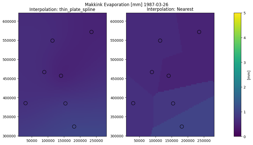
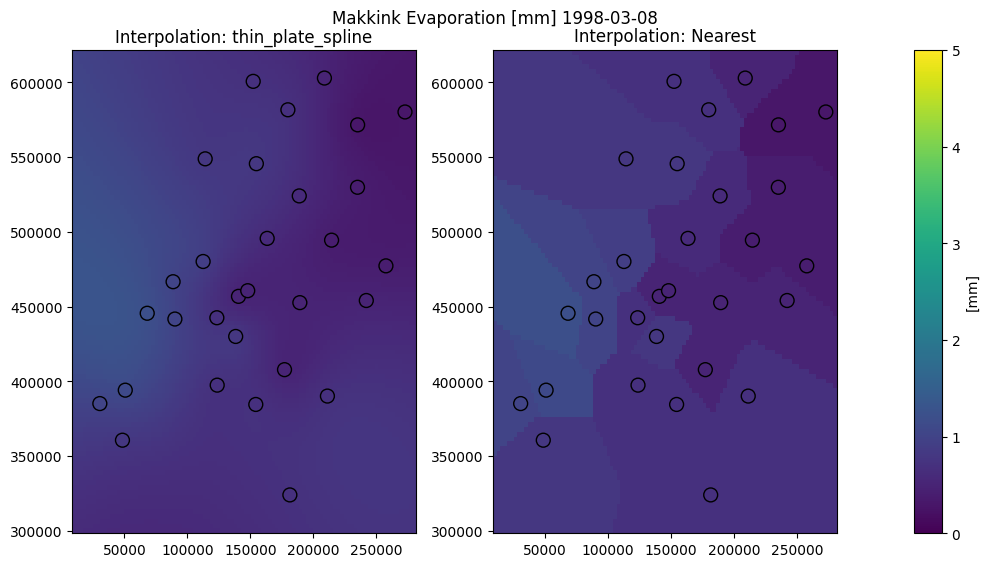
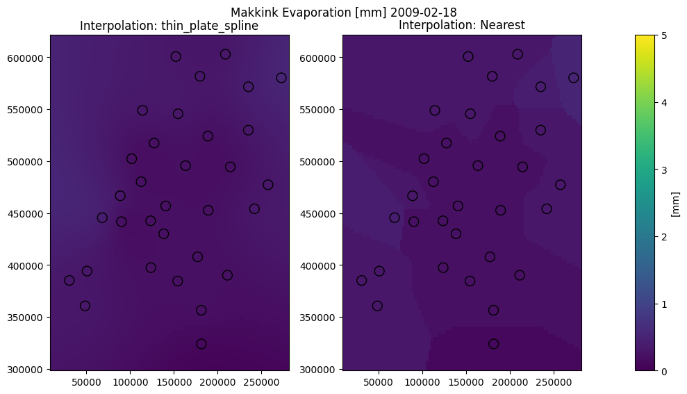
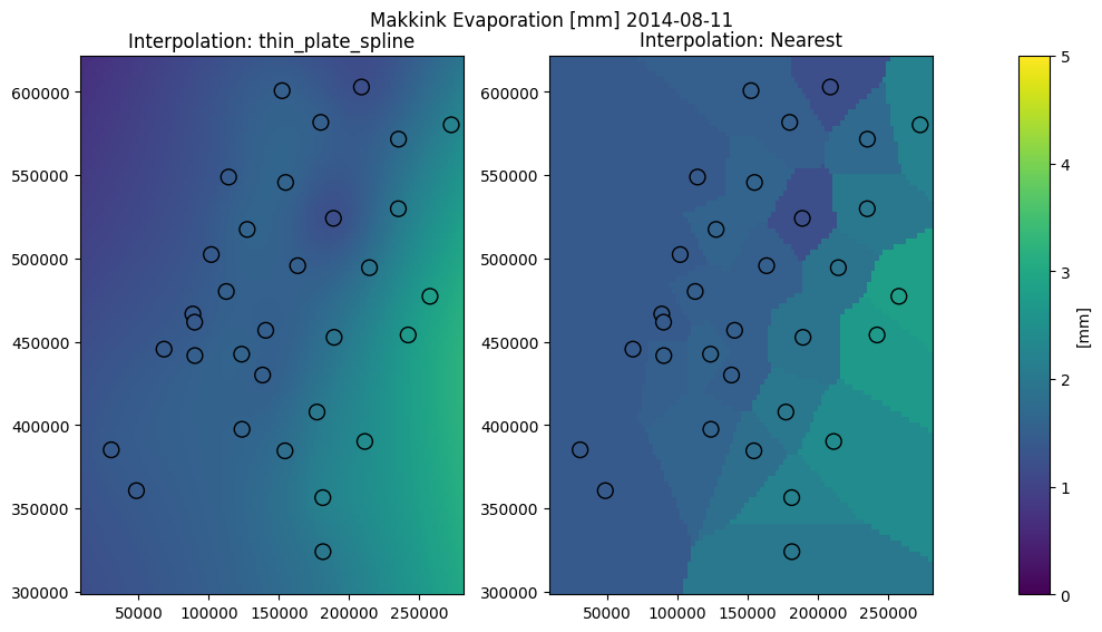
According to the KNMI, thin plate spline is the best way to interpolate Makkink evaporation. Thats also how they provide the gridded Makkink evaporation :
Evaporation Dataset - gridded daily Makkink evaporation for the Netherlands
Interpolation of Makkink evaporation in the Netherlands - Paul Hiemstra and Raymond Sluiter (2011)
[28]:
xy = stns.loc[df.columns, ["x", "y"]]

for idx in tqdm(df.index[0 : len(df) : 2000]):
    # get all stations with values for this date
    val = df.loc[idx].dropna() * 1000  # mm
    # get stations for this date
    coor = xy.loc[val.index].to_numpy()
    if (
        len(val) < 3
    ):  # if there are less than 3 stations, thin plate spline does not work
        # options: linear, multiquadric, gaussian,
        kernel = "linear"

    else:
        kernel = "thin_plate_spline"
        # options:
        # 'inverse_quadratic', 'linear', 'multiquadric', 'gaussian',
        # 'inverse_multiquadric', 'cubic', 'quintic', 'thin_plate_spline'

    # create an scipy interpolator
    rbf = RBFInterpolator(coor, val.to_numpy(), epsilon=1, kernel=kernel)

    nea = NearestNDInterpolator(coor, val.to_numpy())

    # interpolate on grid of the Netherlands
    grid = np.mgrid[10000:280000:100j, 300000:620000:100j]
    grid2 = grid.reshape(2, -1).T  # interpolator only takes array [[x0, y0],
    #  [x1, y1]]
    val_rbf = rbf.__call__(grid2).reshape(100, 100)
    val_nea = nea.__call__(grid2).reshape(100, 100)

    # create figure
    fig, ax = plt.subplot_mosaic("AAAABBBBC", figsize=(10, 5.925))
    fig.suptitle(f"Makkink Evaporation [mm] {idx.date()}", y=0.95)
    vmin = 0
    vmax = 5

    ax["A"].set_title(f"Interpolation: {kernel}")
    ax["A"].pcolormesh(grid[0], grid[1], val_rbf, vmin=vmin, vmax=vmax)
    ax["B"].set_title("Interpolation: Nearest")
    ax["B"].pcolormesh(grid[0], grid[1], val_nea, vmin=vmin, vmax=vmax)
    ax["A"].scatter(*coor.T, c=val, s=100, ec="k", vmin=vmin, vmax=vmax)
    p = ax["B"].scatter(*coor.T, c=val, s=100, ec="k", vmin=vmin, vmax=vmax)
    cb = fig.colorbar(p, cax=ax["C"])
    cb.set_label("[mm]")
    fig.tight_layout()
100%|██████████| 6/6 [00:00<00:00, 11.01it/s]

The same method is implemented in Hydropandas for an ObsCollection.
[29]:
sd = "2022-01-01"
ed = "2022-12-31"
oc = hpd.read_knmi(
    stns=stns.index, starts=sd, ends=ed, meteo_vars=["EV24"], raise_exceptions=False
)
oc_et = oc.interpolate(xy=[(100000, 330000)])
eti = oc_et.iloc[0].obs
eti
INFO:hydropandas.io.knmi.get_knmi_obs:get data from station 210 and variable EV24 from 2022-01-01 to 2022-12-31
WARNING:hydropandas.io.knmi.parse_data:No columns to parse from file. Returning empty DataFrame.
WARNING:hydropandas.io.knmi.get_timeseries_stn:No data for meteo_var='EV24' at stn=210 betweenstart=Timestamp('2022-01-01 00:00:00') and end=Timestamp('2022-12-31 00:00:00').
INFO:hydropandas.io.knmi.get_knmi_obs:get data from station 215 and variable EV24 from 2022-01-01 to 2022-12-31
INFO:hydropandas.io.knmi.get_knmi_obs:get data from station 235 and variable EV24 from 2022-01-01 to 2022-12-31
INFO:hydropandas.io.knmi.get_knmi_obs:get data from station 240 and variable EV24 from 2022-01-01 to 2022-12-31
INFO:hydropandas.io.knmi.get_knmi_obs:get data from station 249 and variable EV24 from 2022-01-01 to 2022-12-31
INFO:hydropandas.io.knmi.get_knmi_obs:get data from station 251 and variable EV24 from 2022-01-01 to 2022-12-31
INFO:hydropandas.io.knmi.get_knmi_obs:get data from station 257 and variable EV24 from 2022-01-01 to 2022-12-31
INFO:hydropandas.io.knmi.get_knmi_obs:get data from station 260 and variable EV24 from 2022-01-01 to 2022-12-31
INFO:hydropandas.io.knmi.get_knmi_obs:get data from station 265 and variable EV24 from 2022-01-01 to 2022-12-31
WARNING:hydropandas.io.knmi.parse_data:No columns to parse from file. Returning empty DataFrame.
WARNING:hydropandas.io.knmi.get_timeseries_stn:No data for meteo_var='EV24' at stn=265 betweenstart=Timestamp('2022-01-01 00:00:00') and end=Timestamp('2022-12-31 00:00:00').
INFO:hydropandas.io.knmi.get_knmi_obs:get data from station 267 and variable EV24 from 2022-01-01 to 2022-12-31
INFO:hydropandas.io.knmi.get_knmi_obs:get data from station 269 and variable EV24 from 2022-01-01 to 2022-12-31
INFO:hydropandas.io.knmi.get_knmi_obs:get data from station 270 and variable EV24 from 2022-01-01 to 2022-12-31
INFO:hydropandas.io.knmi.get_knmi_obs:get data from station 273 and variable EV24 from 2022-01-01 to 2022-12-31
INFO:hydropandas.io.knmi.get_knmi_obs:get data from station 275 and variable EV24 from 2022-01-01 to 2022-12-31
INFO:hydropandas.io.knmi.get_knmi_obs:get data from station 277 and variable EV24 from 2022-01-01 to 2022-12-31
INFO:hydropandas.io.knmi.get_knmi_obs:get data from station 278 and variable EV24 from 2022-01-01 to 2022-12-31
INFO:hydropandas.io.knmi.get_knmi_obs:get data from station 279 and variable EV24 from 2022-01-01 to 2022-12-31
INFO:hydropandas.io.knmi.get_knmi_obs:get data from station 280 and variable EV24 from 2022-01-01 to 2022-12-31
INFO:hydropandas.io.knmi.get_knmi_obs:get data from station 283 and variable EV24 from 2022-01-01 to 2022-12-31
INFO:hydropandas.io.knmi.get_knmi_obs:get data from station 286 and variable EV24 from 2022-01-01 to 2022-12-31
INFO:hydropandas.io.knmi.get_knmi_obs:get data from station 290 and variable EV24 from 2022-01-01 to 2022-12-31
INFO:hydropandas.io.knmi.get_knmi_obs:get data from station 310 and variable EV24 from 2022-01-01 to 2022-12-31
INFO:hydropandas.io.knmi.get_knmi_obs:get data from station 319 and variable EV24 from 2022-01-01 to 2022-12-31
INFO:hydropandas.io.knmi.get_knmi_obs:get data from station 323 and variable EV24 from 2022-01-01 to 2022-12-31
INFO:hydropandas.io.knmi.get_knmi_obs:get data from station 330 and variable EV24 from 2022-01-01 to 2022-12-31
INFO:hydropandas.io.knmi.get_knmi_obs:get data from station 344 and variable EV24 from 2022-01-01 to 2022-12-31
INFO:hydropandas.io.knmi.get_knmi_obs:get data from station 348 and variable EV24 from 2022-01-01 to 2022-12-31
INFO:hydropandas.io.knmi.get_knmi_obs:get data from station 350 and variable EV24 from 2022-01-01 to 2022-12-31
INFO:hydropandas.io.knmi.get_knmi_obs:get data from station 356 and variable EV24 from 2022-01-01 to 2022-12-31
INFO:hydropandas.io.knmi.get_knmi_obs:get data from station 370 and variable EV24 from 2022-01-01 to 2022-12-31
INFO:hydropandas.io.knmi.get_knmi_obs:get data from station 375 and variable EV24 from 2022-01-01 to 2022-12-31
INFO:hydropandas.io.knmi.get_knmi_obs:get data from station 377 and variable EV24 from 2022-01-01 to 2022-12-31
INFO:hydropandas.io.knmi.get_knmi_obs:get data from station 380 and variable EV24 from 2022-01-01 to 2022-12-31
INFO:hydropandas.io.knmi.get_knmi_obs:get data from station 391 and variable EV24 from 2022-01-01 to 2022-12-31
[29]:
hydropandas.EvaporationObs
| 100000_330000 | |
|---|---|
| x | 100000 |
| y | 330000 |
| location | |
| filename | |
| source | interpolation |
| unit | |
| station | NaN |
| meteo_var | EV24 |
| 100000_330000 | |
|---|---|
| YYYYMMDD | |
| 2022-01-01 01:00:00 | 0.000254 |
| 2022-01-02 01:00:00 | 0.000570 |
| 2022-01-03 01:00:00 | 0.000330 |
| 2022-01-04 01:00:00 | 0.000142 |
| 2022-01-05 01:00:00 | 0.000157 |
| ... | ... |
| 2022-12-27 01:00:00 | 0.000151 |
| 2022-12-28 01:00:00 | 0.000260 |
| 2022-12-29 01:00:00 | 0.000101 |
| 2022-12-30 01:00:00 | 0.000141 |
| 2022-12-31 01:00:00 | 0.000077 |
365 rows × 1 columns
[30]:
etn = hpd.MeteoObs.from_knmi(
    xy=(100000, 330000), start=sd, end=ed, meteo_var="EV24", fill_missing_obs=True
)
etn
INFO:hydropandas.io.knmi.get_knmi_obs:get KNMI data from station nearest to coordinates (100000, 330000) and meteovariable EV24
[30]:
hydropandas.MeteoObs
| EV24_WESTDORPE_319 | |
|---|---|
| x | 48425.362049 |
| y | 360618.713456 |
| location | |
| filename | |
| source | KNMI |
| unit | m |
| station | 319 |
| meteo_var | EV24 |
| EV24 | station | |
|---|---|---|
| 2022-01-01 01:00:00 | 0.0002 | 319 |
| 2022-01-02 01:00:00 | 0.0005 | 319 |
| 2022-01-03 01:00:00 | 0.0004 | 319 |
| 2022-01-04 01:00:00 | 0.0002 | 319 |
| 2022-01-05 01:00:00 | 0.0002 | 319 |
| ... | ... | ... |
| 2022-12-27 01:00:00 | 0.0003 | 319 |
| 2022-12-28 01:00:00 | 0.0003 | 319 |
| 2022-12-29 01:00:00 | 0.0001 | 319 |
| 2022-12-30 01:00:00 | 0.0002 | 319 |
| 2022-12-31 01:00:00 | 0.0001 | 319 |
365 rows × 2 columns
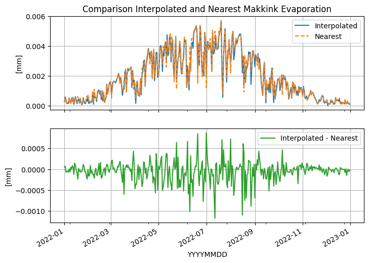
As can be seen, for one location the interpolation method is significantly slower. Lets see how the values compare for a time series.
[31]:
fig, ax = plt.subplots(2, 1, figsize=(8, 6), sharex=True)
eti.plot(ax=ax[0])
etn.plot(ax=ax[0], linestyle="--", color="C1")
ax[0].set_title("Comparison Interpolated and Nearest Makkink Evaporation")
ax[0].set_ylabel("[mm]")
ax[0].grid()
ax[0].legend(["Interpolated", "Nearest"])

(eti.squeeze() - etn["EV24"].squeeze()).plot(ax=ax[1], color="C2")
ax[1].set_ylabel("[mm]")
ax[1].grid()
ax[1].legend(["Interpolated - Nearest"])
[31]:
<matplotlib.legend.Legend at 0x7f755165b9b0>
The interpolated evaporation can also be collected for multiple points (using x and y in a list of DataFrame) in an ObsCollection
[32]:
oc_et = oc.interpolate(xy=[(100000, 320000), (100000, 330000), (100000, 340000)])
oc_et
[32]:
| x | y | location | filename | source | unit | station | meteo_var | obs | |
|---|---|---|---|---|---|---|---|---|---|
| name | |||||||||
| 100000_320000 | 100000 | 320000 | interpolation | NaN | EV24 | EvaporationObs 100000_320000 -----metadata----... | |||
| 100000_330000 | 100000 | 330000 | interpolation | NaN | EV24 | EvaporationObs 100000_330000 -----metadata----... | |||
| 100000_340000 | 100000 | 340000 | interpolation | NaN | EV24 | EvaporationObs 100000_340000 -----metadata----... |
The interpolation method is slow at first, but if collected for many different locations the time penalty is not that significant anymore.