Reading groundwater observations
This notebook introduces how to use the hydropandas package to read, process and visualise groundwater data from Dino and Bro databases.
Notebook contents
Write ObsCollections
[1]:
import contextily as ctx
from IPython.display import HTML

import hydropandas as hpd
[2]:
hpd.util.get_color_logger("INFO")
[2]:
<RootLogger root (INFO)>
GroundwaterObs
The hydropandas package has several functions to read groundwater observations at a measurement well. These include reading data from:
dino (from csv-files).
bro (using the bro-api)
fews (xml dumps from the fews database)
wiski (dumps from the wiski database)
[3]:
# reading a dino csv file
path = "data/Grondwaterstanden_Put/B33F0080001_1.csv"
gw_dino = hpd.GroundwaterObs.from_dino(path=path)
gw_dino
INFO:hydropandas.io.dino.read_dino_groundwater_csv:reading -> B33F0080001_1
[3]:
hydropandas.GroundwaterObs
| B33F0080-001 | |
|---|---|
| x | 213260.0 |
| y | 473900.0 |
| location | B33F0080 |
| filename | B33F0080001_1 |
| source | dino |
| unit | m NAP |
| tube_nr | 1.0 |
| screen_top | 3.85 |
| screen_bottom | 2.85 |
| ground_level | 6.92 |
| tube_top | 7.18 |
| metadata_available | True |
| stand_m_tov_nap | locatie | filternummer | stand_cm_tov_mp | stand_cm_tov_mv | stand_cm_tov_nap | bijzonderheid | opmerking | tube_top | ground_level | |
|---|---|---|---|---|---|---|---|---|---|---|
| 1972-11-28 | 5.76 | B33F0080 | 1 | 141 | 109 | 576 | NaN | NaN | 7.17 | 6.85 |
| 1972-12-07 | 5.77 | B33F0080 | 1 | 140 | 108 | 577 | NaN | NaN | 7.17 | 6.85 |
| 1972-12-14 | 5.70 | B33F0080 | 1 | 147 | 115 | 570 | NaN | NaN | 7.17 | 6.85 |
| 1972-12-21 | 5.64 | B33F0080 | 1 | 153 | 121 | 564 | NaN | NaN | 7.17 | 6.85 |
| 1972-12-28 | 5.57 | B33F0080 | 1 | 160 | 128 | 557 | NaN | NaN | 7.17 | 6.85 |
| ... | ... | ... | ... | ... | ... | ... | ... | ... | ... | ... |
| 2015-06-13 | 5.42 | B33F0080 | 1 | 176 | 150 | 542 | NaN | NaN | 7.18 | 6.92 |
| 2015-06-14 | 5.42 | B33F0080 | 1 | 176 | 150 | 542 | NaN | NaN | 7.18 | 6.92 |
| 2015-06-15 | 5.40 | B33F0080 | 1 | 178 | 152 | 540 | NaN | NaN | 7.18 | 6.92 |
| 2015-06-16 | 5.40 | B33F0080 | 1 | 178 | 152 | 540 | NaN | NaN | 7.18 | 6.92 |
| 2015-06-17 | 5.40 | B33F0080 | 1 | 178 | 152 | 540 | NaN | NaN | 7.18 | 6.92 |
3988 rows × 10 columns
[4]:
# reading the same filter from using the bro api. Specify a groundwater monitoring id (GMW00...) and a filter number (1)
gw_bro = hpd.GroundwaterObs.from_bro("GMW000000041261", 1)
Now we have an GroundwaterObs object named gw_bro and gw_dino. Both objects are from the same measurement well in different databases. A GroundwaterObs object inherits from a pandas DataFrame and has the same attributes and methods.
[5]:
gw_bro.describe()
[5]:
| values | |
|---|---|
| count | 66411.000000 |
| mean | 5.562630 |
| std | 0.222262 |
| min | 4.913000 |
| 25% | 5.380000 |
| 50% | 5.569000 |
| 75% | 5.721000 |
| max | 6.397000 |
[6]:
gw_bro
[6]:
hydropandas.GroundwaterObs
| GMW000000041261_1 | |
|---|---|
| x | 213268.000067 |
| y | 473909.999949 |
| location | GMW000000041261 |
| filename | |
| source | BRO |
| unit | m NAP |
| tube_nr | 1 |
| screen_top | 4.05 |
| screen_bottom | 3.05 |
| ground_level | 6.9 |
| tube_top | 7.173 |
| metadata_available | True |
| values | qualifier | |
|---|---|---|
| 1972-11-28 00:00:00 | 5.763 | goedgekeurd |
| 1972-12-07 00:00:00 | 5.773 | goedgekeurd |
| 1972-12-14 00:00:00 | 5.703 | goedgekeurd |
| 1972-12-21 00:00:00 | 5.643 | goedgekeurd |
| 1972-12-28 00:00:00 | 5.573 | goedgekeurd |
| ... | ... | ... |
| 2021-10-08 07:00:00 | 5.486 | goedgekeurd |
| 2021-10-08 08:00:00 | 5.485 | goedgekeurd |
| 2021-10-08 09:00:00 | 5.486 | goedgekeurd |
| 2021-10-08 09:47:00 | 5.491 | goedgekeurd |
| 2021-10-08 10:00:00 | 5.485 | goedgekeurd |
66411 rows × 2 columns
[7]:
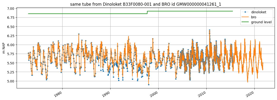
ax = gw_dino["stand_m_tov_nap"].plot(
    label="dinoloket", figsize=(14, 5), legend=True, marker=".", lw=0.2
)
gw_bro["values"].plot(ax=ax, label="bro", legend=True, ylabel=gw_bro.unit)
gw_dino["ground_level"].plot(
    ax=ax,
    label="ground level",
    legend=True,
    grid=True,
    color="green",
    ylabel=gw_dino.unit,
)

ax.set_title(f"same tube from Dinoloket {gw_dino.name} and BRO id {gw_bro.name}")
[7]:
Text(0.5, 1.0, 'same tube from Dinoloket B33F0080-001 and BRO id GMW000000041261_1')
GroundwaterObs Attributes
Besides the standard DataFrame attributes a GroundwaterObs has the following additional attributes:
x, y: x- and y-coordinates of the observation point
name: str with the name
filename: str with the filename (only available when the data was loaded from a file)
monitoring_well: the name of the monitoring_well. One monitoring well can have multiple tubes.
tube_nr: the number of the tube. The combination of monitoring_well and tube_nr should be unique
screen_top: the top of the tube screen (bovenkant filter in Dutch)
screen_bottom: the bottom of the tube screen (onderkant filter in Dutch)
ground_level: surface level (maaiveld in Dutch)
tube_top: the top of the tube
metadata_available: boolean indicating whether metadata is available for this observation point
meta: dictionary with additional metadata
When dowloading from Dinoloket all levels are in meters NAP.
[8]:
print(gw_bro)
GroundwaterObs GMW000000041261_1
-----metadata------
name : GMW000000041261_1
x : 213268.00006656803
y : 473909.9999492651
location : GMW000000041261
filename :
source : BRO
unit : m NAP
tube_nr : 1
screen_top : 4.05
screen_bottom : 3.05
ground_level : 6.9
tube_top : 7.173
metadata_available : True

-----time series------
                     values    qualifier
1972-11-28 00:00:00   5.763  goedgekeurd
1972-12-07 00:00:00   5.773  goedgekeurd
1972-12-14 00:00:00   5.703  goedgekeurd
1972-12-21 00:00:00   5.643  goedgekeurd
1972-12-28 00:00:00   5.573  goedgekeurd
...                     ...          ...
2021-10-08 07:00:00   5.486  goedgekeurd
2021-10-08 08:00:00   5.485  goedgekeurd
2021-10-08 09:00:00   5.486  goedgekeurd
2021-10-08 09:47:00   5.491  goedgekeurd
2021-10-08 10:00:00   5.485  goedgekeurd

[66411 rows x 2 columns]
GroundwaterObs methods
Besides the standard DataFrame methods a GroundwaterObs has additional methods. This methods are accessible through submodules:
geo.get_lat_lon(), to obtain latitude and longitudegwobs.get_modellayer(), to obtain the modellayer of a modflow model using the filter depthstats.get_seasonal_stat(), to obtain seasonal statisticsstats.obs_per_year(), to obtain the number of observations per yearstats.consecutive_obs_years(), to obtain the number of consecutive years with more than a minimum number of observationsplots.interactive_plot(), to obtain a bokeh plot
Get latitude and longitude with gw.geo.get_lat_lon():
[9]:
print(f"latitude and longitude -> {gw_bro.geo.get_lat_lon()}")
latitude and longitude -> (52.25014706691896, 6.2404799462571825)
[10]:
gw_bro.stats.get_seasonal_stat(stat="mean")
[10]:
| winter_mean | summer_mean | |
|---|---|---|
| GMW000000041261_1 | 5.723791 | 5.40682 |
[11]:
p = gw_bro.plots.interactive_plot("figure")
HTML(filename="figure/{}.html".format(gw_bro.name))
[11]:
ObsCollections
ObsCollections are a combination of multiple observation objects. The easiest way to construct an ObsCollections is from a list of observation objects.
[12]:
path1 = "data/Grondwaterstanden_Put/B33F0080001_1.csv"
path2 = "data/Grondwaterstanden_Put/B33F0133001_1.csv"
gw1 = hpd.GroundwaterObs.from_dino(path=path1)
gw2 = hpd.GroundwaterObs.from_dino(path=path2)

# create ObsCollection
oc = hpd.ObsCollection([gw1, gw2], name="Dino groundwater")
oc
INFO:hydropandas.io.dino.read_dino_groundwater_csv:reading -> B33F0080001_1
INFO:hydropandas.io.dino.read_dino_groundwater_csv:reading -> B33F0133001_1
[12]:
| x | y | location | filename | source | unit | tube_nr | screen_top | screen_bottom | ground_level | tube_top | metadata_available | obs | |
|---|---|---|---|---|---|---|---|---|---|---|---|---|---|
| name | |||||||||||||
| B33F0080-001 | 213260.0 | 473900.0 | B33F0080 | B33F0080001_1 | dino | m NAP | 1.0 | 3.85 | 2.85 | 6.92 | 7.18 | True | GroundwaterObs B33F0080-001 -----metadata-----... |
| B33F0133-001 | 210400.0 | 473366.0 | B33F0133 | B33F0133001_1 | dino | m NAP | 1.0 | -67.50 | -70.00 | 6.50 | 7.14 | True | GroundwaterObs B33F0133-001 -----metadata-----... |
Now we have an ObsCollection object named oc. The ObsCollection contains all the data from the two GroundwaterObs objects. It also stores a reference to the GroundwaterObs objects in the ‘obs’ column. An ObsCollection object also inherits from a pandas DataFrame and has the same attributes and methods.
[13]:
# get columns
oc.columns
[13]:
Index(['x', 'y', 'location', 'filename', 'source', 'unit', 'tube_nr',
       'screen_top', 'screen_bottom', 'ground_level', 'tube_top',
       'metadata_available', 'obs'],
      dtype='object')
[14]:
# get individual GroundwaterObs object from an ObsCollection
o = oc.loc["B33F0133-001", "obs"]
o
[14]:
hydropandas.GroundwaterObs
| B33F0133-001 | |
|---|---|
| x | 210400.0 |
| y | 473366.0 |
| location | B33F0133 |
| filename | B33F0133001_1 |
| source | dino |
| unit | m NAP |
| tube_nr | 1.0 |
| screen_top | -67.5 |
| screen_bottom | -70.0 |
| ground_level | 6.5 |
| tube_top | 7.14 |
| metadata_available | True |
| stand_m_tov_nap | locatie | filternummer | stand_cm_tov_mp | stand_cm_tov_mv | stand_cm_tov_nap | bijzonderheid | opmerking | tube_top | |
|---|---|---|---|---|---|---|---|---|---|
| 1989-12-14 | 1.20 | B33F0133 | 1 | 582.0 | 530.0 | 120.0 | NaN | NaN | 7.02 |
| 1990-01-15 | 1.57 | B33F0133 | 1 | 545.0 | 493.0 | 157.0 | NaN | NaN | 7.02 |
| 1990-01-29 | 1.70 | B33F0133 | 1 | 532.0 | 480.0 | 170.0 | NaN | NaN | 7.02 |
| 1990-02-14 | 1.53 | B33F0133 | 1 | 549.0 | 497.0 | 153.0 | NaN | NaN | 7.02 |
| 1990-03-01 | 1.56 | B33F0133 | 1 | 546.0 | 494.0 | 156.0 | NaN | NaN | 7.02 |
| ... | ... | ... | ... | ... | ... | ... | ... | ... | ... |
| 2011-01-14 | 3.57 | B33F0133 | 1 | 357.0 | 293.0 | 357.0 | NaN | NaN | 7.14 |
| 2011-01-15 | 3.60 | B33F0133 | 1 | 354.0 | 290.0 | 360.0 | NaN | NaN | 7.14 |
| 2011-01-16 | 3.61 | B33F0133 | 1 | 353.0 | 289.0 | 361.0 | NaN | NaN | 7.14 |
| 2011-01-17 | 3.61 | B33F0133 | 1 | 353.0 | 289.0 | 361.0 | NaN | NaN | 7.14 |
| 2011-01-18 | 3.63 | B33F0133 | 1 | 351.0 | 287.0 | 363.0 | NaN | NaN | 7.14 |
2212 rows × 9 columns
[15]:
# get statistics
oc.describe()
[15]:
| x | y | tube_nr | screen_top | screen_bottom | ground_level | tube_top | |
|---|---|---|---|---|---|---|---|
| count | 2.000000 | 2.000000 | 2.0 | 2.000000 | 2.000000 | 2.000000 | 2.000000 |
| mean | 211830.000000 | 473633.000000 | 1.0 | -31.825000 | -33.575000 | 6.710000 | 7.160000 |
| std | 2022.325394 | 377.595021 | 0.0 | 50.452069 | 51.512729 | 0.296985 | 0.028284 |
| min | 210400.000000 | 473366.000000 | 1.0 | -67.500000 | -70.000000 | 6.500000 | 7.140000 |
| 25% | 211115.000000 | 473499.500000 | 1.0 | -49.662500 | -51.787500 | 6.605000 | 7.150000 |
| 50% | 211830.000000 | 473633.000000 | 1.0 | -31.825000 | -33.575000 | 6.710000 | 7.160000 |
| 75% | 212545.000000 | 473766.500000 | 1.0 | -13.987500 | -15.362500 | 6.815000 | 7.170000 |
| max | 213260.000000 | 473900.000000 | 1.0 | 3.850000 | 2.850000 | 6.920000 | 7.180000 |
ObsCollection methods
Besides the methods of a pandas DataFrame an ObsCollection has additional methods stored in submodules.
geo:
get_bounding_box-> get a tuple with (xmin, ymin, xmax, ymax)get_extent-> get a tule with (xmin, xmax, ymin, ymax)get_lat_lon-> to get the lattitudes and longitudes from the x and y coordinateswithin_polygon-> to select only the observations that lie within a polygon
gwobs:
set_tube_nr-> to set the tube numbers based on the tube screen depth when there are multiple tubes at one monitoring wellset_tube_nr_monitoring_well-> find out which observations are at the same location with a different screen depth. Set monitoring_well and tube_nr attributes accordingly.
plots:
interactive_figures-> create bokeh figures for each observation point.interactive_map-> create a folium map with observation points and bokeh figures for each observation point.section_plot-> create a plot of multiple observations and a plot of the well layout.
stats:
get_first_last_obs_date()-> get the first and the last date of the observations for each observation pointget_no_of_observations()-> get the number of observationsget_seasonal_stat()-> get seasonal stats of the observations
E.g. get the bounding box with gw.geo.get_bounding_box():
[16]:
print(f"bounding box -> {oc.geo.get_bounding_box()}")
bounding box -> (np.float64(210400.0), np.float64(473366.0), np.float64(213260.0), np.float64(473900.0))
[17]:
oc.geo.set_lat_lon()
oc.plots.interactive_map(plot_dir="figure", popup_width=300)
[17]:
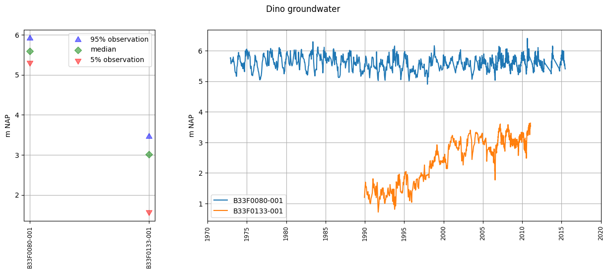
We can get an overview of the well layout and observations via plots.section_plot:
[18]:
oc.plots.section_plot()
INFO:hydropandas.extensions.plots.section_plot:created sectionplot -> B33F0080-001
INFO:hydropandas.extensions.plots.section_plot:created sectionplot -> B33F0133-001
[18]:
(<Figure size 1500x500 with 2 Axes>,
 [<Axes: ylabel='m NAP'>, <Axes: ylabel='m NAP'>])
ObsCollection Attributes
An ObsCollection also has additional attributes:
name, a str with the name of the collection
meta, a dictionary with additional metadata
[19]:
print(f"name is -> {oc.name}")
print(f"meta is -> {oc.meta}")
name is -> Dino groundwater
meta is -> {}
Read ObsCollections
Instead of creating the ObsCollection from a list of observation objects. It is also possible to read the data from a source into an ObsCollection at once. The following sources can be read as an ObsCollection:
bro (using the api)
dino (from files)
fews (dumps from the fews database)
wiski (dumps from the wiski database)
menyanthes (a .men file)
modflow (from the heads of a modflow model)
imod (from the heads of an imod model)
This notebook won’t go into detail on all the sources that can be read. Only the two options for reading data from Dino and BRO are shown below.
[20]:
# read using a .zip file with data
dinozip = "data/dino.zip"
dino_gw = hpd.read_dino(
    dirname=dinozip, subdir="Grondwaterstanden_Put", suffix="1.csv", keep_all_obs=False
)
dino_gw
INFO:hydropandas.io.dino.read_dino_groundwater_csv:reading -> Grondwaterstanden_Put/B02H0092001_1.csv
WARNING:hydropandas.io.dino.read_dino_groundwater_csv:no NAP measurements available -> Grondwaterstanden_Put/B02H0092001_1.csv
INFO:hydropandas.io.dino.read_dino_groundwater_csv:reading -> Grondwaterstanden_Put/B02H1007001_1.csv
WARNING:hydropandas.io.dino.read_dino_groundwater_csv:no NAP measurements available -> Grondwaterstanden_Put/B02H1007001_1.csv
INFO:hydropandas.io.dino.read_dino_groundwater_csv:reading -> Grondwaterstanden_Put/B04D0032002_1.csv
WARNING:hydropandas.io.dino.read_dino_groundwater_csv:could not read metadata -> Grondwaterstanden_Put/B04D0032002_1.csv
WARNING:hydropandas.io.dino.read_dino_groundwater_csv:no NAP measurements available -> Grondwaterstanden_Put/B04D0032002_1.csv
INFO:root.get_dino_obs:not added to collection -> Grondwaterstanden_Put/B04D0032002_1.csv
INFO:hydropandas.io.dino.read_dino_groundwater_csv:reading -> Grondwaterstanden_Put/B27D0260001_1.csv
WARNING:hydropandas.io.dino.read_dino_groundwater_csv:could not read metadata -> Grondwaterstanden_Put/B27D0260001_1.csv
WARNING:hydropandas.io.dino.read_dino_groundwater_csv:no NAP measurements available -> Grondwaterstanden_Put/B27D0260001_1.csv
INFO:root.get_dino_obs:not added to collection -> Grondwaterstanden_Put/B27D0260001_1.csv
INFO:hydropandas.io.dino.read_dino_groundwater_csv:reading -> Grondwaterstanden_Put/B33F0080001_1.csv
INFO:hydropandas.io.dino.read_dino_groundwater_csv:reading -> Grondwaterstanden_Put/B33F0080002_1.csv
INFO:hydropandas.io.dino.read_dino_groundwater_csv:reading -> Grondwaterstanden_Put/B33F0133001_1.csv
INFO:hydropandas.io.dino.read_dino_groundwater_csv:reading -> Grondwaterstanden_Put/B33F0133002_1.csv
INFO:hydropandas.io.dino.read_dino_groundwater_csv:reading -> Grondwaterstanden_Put/B37A0112001_1.csv
WARNING:hydropandas.io.dino.read_dino_groundwater_csv:could not read metadata -> Grondwaterstanden_Put/B37A0112001_1.csv
WARNING:hydropandas.io.dino.read_dino_groundwater_csv:could not read measurements -> Grondwaterstanden_Put/B37A0112001_1.csv
INFO:root.get_dino_obs:not added to collection -> Grondwaterstanden_Put/B37A0112001_1.csv
INFO:hydropandas.io.dino.read_dino_groundwater_csv:reading -> Grondwaterstanden_Put/B42B0003001_1.csv
INFO:hydropandas.io.dino.read_dino_groundwater_csv:reading -> Grondwaterstanden_Put/B42B0003002_1.csv
INFO:hydropandas.io.dino.read_dino_groundwater_csv:reading -> Grondwaterstanden_Put/B42B0003003_1.csv
INFO:hydropandas.io.dino.read_dino_groundwater_csv:reading -> Grondwaterstanden_Put/B42B0003004_1.csv
INFO:hydropandas.io.dino.read_dino_groundwater_csv:reading -> Grondwaterstanden_Put/B58A0092004_1.csv
INFO:hydropandas.io.dino.read_dino_groundwater_csv:reading -> Grondwaterstanden_Put/B58A0092005_1.csv
INFO:hydropandas.io.dino.read_dino_groundwater_csv:reading -> Grondwaterstanden_Put/B58A0102001_1.csv
INFO:hydropandas.io.dino.read_dino_groundwater_csv:reading -> Grondwaterstanden_Put/B58A0167001_1.csv
INFO:hydropandas.io.dino.read_dino_groundwater_csv:reading -> Grondwaterstanden_Put/B58A0212001_1.csv
INFO:hydropandas.io.dino.read_dino_groundwater_csv:reading -> Grondwaterstanden_Put/B22D0155001_1.csv
[20]:
| x | y | location | filename | source | unit | tube_nr | screen_top | screen_bottom | ground_level | tube_top | metadata_available | obs | |
|---|---|---|---|---|---|---|---|---|---|---|---|---|---|
| name | |||||||||||||
| B02H0092-001 | 219890.0 | 600030.0 | B02H0092 | Grondwaterstanden_Put/B02H0092001_1.csv | dino | m NAP | 1.0 | NaN | NaN | NaN | NaN | True | GroundwaterObs B02H0092-001 -----metadata-----... |
| B02H1007-001 | 219661.0 | 600632.0 | B02H1007 | Grondwaterstanden_Put/B02H1007001_1.csv | dino | m NAP | 1.0 | NaN | NaN | 1.92 | NaN | True | GroundwaterObs B02H1007-001 -----metadata-----... |
| B33F0080-001 | 213260.0 | 473900.0 | B33F0080 | Grondwaterstanden_Put/B33F0080001_1.csv | dino | m NAP | 1.0 | 3.85 | 2.85 | 6.92 | 7.18 | True | GroundwaterObs B33F0080-001 -----metadata-----... |
| B33F0080-002 | 213260.0 | 473900.0 | B33F0080 | Grondwaterstanden_Put/B33F0080002_1.csv | dino | m NAP | 2.0 | -10.15 | -12.15 | 6.92 | 7.17 | True | GroundwaterObs B33F0080-002 -----metadata-----... |
| B33F0133-001 | 210400.0 | 473366.0 | B33F0133 | Grondwaterstanden_Put/B33F0133001_1.csv | dino | m NAP | 1.0 | -67.50 | -70.00 | 6.50 | 7.14 | True | GroundwaterObs B33F0133-001 -----metadata-----... |
| B33F0133-002 | 210400.0 | 473366.0 | B33F0133 | Grondwaterstanden_Put/B33F0133002_1.csv | dino | m NAP | 2.0 | -104.20 | -106.20 | 6.50 | 7.12 | True | GroundwaterObs B33F0133-002 -----metadata-----... |
| B42B0003-001 | 38165.0 | 413785.0 | B42B0003 | Grondwaterstanden_Put/B42B0003001_1.csv | dino | m NAP | 1.0 | -2.00 | -3.00 | 6.50 | 6.99 | True | GroundwaterObs B42B0003-001 -----metadata-----... |
| B42B0003-002 | 38165.0 | 413785.0 | B42B0003 | Grondwaterstanden_Put/B42B0003002_1.csv | dino | m NAP | 2.0 | -34.00 | -35.00 | 6.50 | 6.99 | True | GroundwaterObs B42B0003-002 -----metadata-----... |
| B42B0003-003 | 38165.0 | 413785.0 | B42B0003 | Grondwaterstanden_Put/B42B0003003_1.csv | dino | m NAP | 3.0 | -60.00 | -61.00 | 6.50 | 6.95 | True | GroundwaterObs B42B0003-003 -----metadata-----... |
| B42B0003-004 | 38165.0 | 413785.0 | B42B0003 | Grondwaterstanden_Put/B42B0003004_1.csv | dino | m NAP | 4.0 | -107.00 | -108.00 | 6.50 | 6.97 | True | GroundwaterObs B42B0003-004 -----metadata-----... |
| B58A0092-004 | 186924.0 | 372026.0 | B58A0092 | Grondwaterstanden_Put/B58A0092004_1.csv | dino | m NAP | 4.0 | -115.23 | -117.23 | 29.85 | 29.61 | True | GroundwaterObs B58A0092-004 -----metadata-----... |
| B58A0092-005 | 186924.0 | 372026.0 | B58A0092 | Grondwaterstanden_Put/B58A0092005_1.csv | dino | m NAP | 5.0 | -134.23 | -137.23 | 29.84 | 29.62 | True | GroundwaterObs B58A0092-005 -----metadata-----... |
| B58A0102-001 | 187900.0 | 373025.0 | B58A0102 | Grondwaterstanden_Put/B58A0102001_1.csv | dino | m NAP | 1.0 | -3.35 | -8.35 | 29.65 | 29.73 | True | GroundwaterObs B58A0102-001 -----metadata-----... |
| B58A0167-001 | 185745.0 | 371095.0 | B58A0167 | Grondwaterstanden_Put/B58A0167001_1.csv | dino | m NAP | 1.0 | 23.33 | 22.33 | 30.50 | 30.21 | True | GroundwaterObs B58A0167-001 -----metadata-----... |
| B58A0212-001 | 183600.0 | 373020.0 | B58A0212 | Grondwaterstanden_Put/B58A0212001_1.csv | dino | m NAP | 1.0 | 26.03 | 25.53 | 28.49 | 28.53 | True | GroundwaterObs B58A0212-001 -----metadata-----... |
| B22D0155-001 | 233830.0 | 502530.0 | B22D0155 | Grondwaterstanden_Put/B22D0155001_1.csv | dino | m NAP | 1.0 | 7.80 | 6.80 | 8.91 | 9.94 | True | GroundwaterObs B22D0155-001 -----metadata-----... |
[21]:
# read from bro using an extent (Schoonhoven zuid-west)
oc = hpd.read_bro(extent=(117850, 118180, 439550, 439900), keep_all_obs=False)
oc
100%|██████████| 5/5 [00:15<00:00, 3.05s/it]
[21]:
| x | y | location | filename | source | unit | tube_nr | screen_top | screen_bottom | ground_level | tube_top | metadata_available | obs | |
|---|---|---|---|---|---|---|---|---|---|---|---|---|---|
| name | |||||||||||||
| GMW000000036319_1 | 117957.010065 | 439698.23595 | GMW000000036319 | BRO | m NAP | 1 | -1.721 | -2.721 | -0.501 | -0.621 | True | GroundwaterObs GMW000000036319_1 -----metadata... | |
| GMW000000036327_1 | 118064.196065 | 439799.96795 | GMW000000036327 | BRO | m NAP | 1 | -0.833 | -1.833 | 0.856 | 0.716 | True | GroundwaterObs GMW000000036327_1 -----metadata... | |
| GMW000000036365_1 | 118127.470065 | 439683.13595 | GMW000000036365 | BRO | m NAP | 1 | -0.429 | -1.428 | 1.371 | 1.221 | True | GroundwaterObs GMW000000036365_1 -----metadata... |
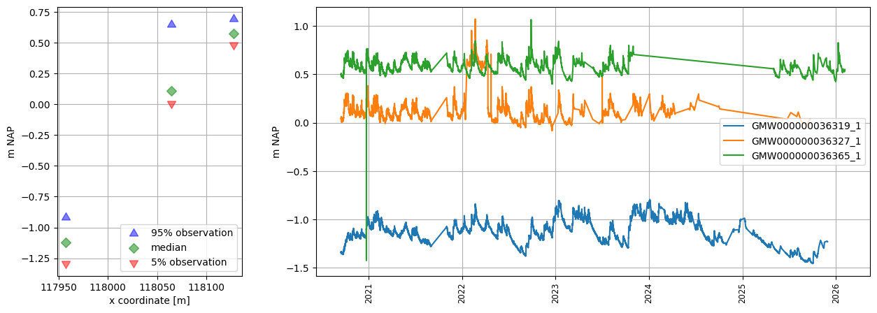
[22]:
# plot wells, use x-coordinate in section plot
oc.plots.section_plot(section_colname_x="x", section_label_x="x coordinate [m]")
INFO:hydropandas.extensions.plots.section_plot:created sectionplot -> GMW000000036319_1
INFO:hydropandas.extensions.plots.section_plot:created sectionplot -> GMW000000036327_1
INFO:hydropandas.extensions.plots.section_plot:created sectionplot -> GMW000000036365_1
[22]:
(<Figure size 1500x500 with 2 Axes>,
 [<Axes: xlabel='x coordinate [m]', ylabel='m NAP'>, <Axes: ylabel='m NAP'>])
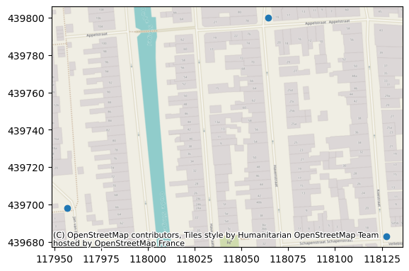
[23]:
ax = oc.to_gdf().plot()
ctx.add_basemap(ax=ax, crs=28992)