Hydropandas Objects: A Comprehensive Guide
Welcome to the core tutorial of HydroPandas! This notebook introduces the two fundamental classes that power all hydrological data analysis in hydropandas: Obs and ObsCollection.
The Obs Class
The Obs class represents a single time series of measurements at a specific location. Think of it as a pandas DataFrame enhanced with metadata and specialized methods. Whether you’re working with groundwater levels, precipitation measurements, or water quality data, Obs objects keep your measurements and metadata together in one organized object.
Available Obs Types:
GroundwaterObs: Groundwater level measurements
WaterQualityObs: Water quality parameters (pH, temperature, conductivity, etc.)
WaterlvlObs: Surface water level measurements
ModelObs: time series from MODFLOW or other hydrological models
MeteoObs: Meteorological observations (general weather data)
PrecipitationObs: Precipitation measurements (specialized MeteoObs)
EvaporationObs: Evaporation measurements (specialized MeteoObs)
The ObsCollection Class
The ObsCollection class manages multiple Obs objects simultaneously. It’s perfect for analyzing data across multiple monitoring locations, comparing time series, or conducting regional studies. Like Obs, it inherits from pandas DataFrame but adds powerful methods for bulk operations and spatial analysis.
Both classes seamlessly integrate with the pandas ecosystem while providing specialized functionality for hydrological data management, quality control, and analysis.
Tutorial Contents
This notebook is organized into two main sections with hands-on examples:
[1]:
import numpy as np
import pandas as pd

import hydropandas as hpd

hpd.util.get_color_logger("INFO")
[1]:
<RootLogger root (INFO)>
Obs
The Obs class is the foundation of hydropandas. Creating an Obs object is very similar to creating a pandas DataFrame, but with enhanced capabilities for hydrological data.
Three Ways to Create Obs Objects
Let’s explore three progressively more complex approaches to creating Obs objects:
Empty Obs - Start with an Empty object with just a name
Metadata-only Obs - Add location and measurement details
Complete Obs - Include both metadata and time series measurements
Each approach serves different purposes in your workflow, from initial setup to full data analysis.
[2]:
# 1. create an empty Obs object
o1 = hpd.Obs(name="my empty obs")
display(o1)
hydropandas.Obs
| my empty obs | |
|---|---|
| x | NaN |
| y | NaN |
| location | |
| filename | |
| source | |
| unit |
[3]:
# 2. create an Obs object with only metadata
o2 = hpd.Obs(
    name="my_observation",
    x=10,
    y=20,
    location="somewhere",
    filename="unknown",
    source="imagination",
    unit="m",
)
display(o2)
hydropandas.Obs
| my_observation | |
|---|---|
| x | 10 |
| y | 20 |
| location | somewhere |
| filename | unknown |
| source | imagination |
| unit | m |
[4]:
# 3. create an Obs object with both metadata and measurements
meas_df = pd.DataFrame(
    index=pd.date_range(start="2020-01-01", periods=10, freq="D"),
    data={"value": np.random.rand(10)},
)
o3 = hpd.Obs(
    meas_df,
    name="smw",
    x=1000,
    y=22220,
    location="somewhere else",
    source="advanced imagination",
    unit="m",
)
display(o3)
hydropandas.Obs
| smw | |
|---|---|
| x | 1000 |
| y | 22220 |
| location | somewhere else |
| filename | |
| source | advanced imagination |
| unit | m |
| value | |
|---|---|
| 2020-01-01 | 0.958142 |
| 2020-01-02 | 0.291446 |
| 2020-01-03 | 0.366914 |
| 2020-01-04 | 0.575771 |
| 2020-01-05 | 0.428153 |
| 2020-01-06 | 0.497021 |
| 2020-01-07 | 0.397704 |
| 2020-01-08 | 0.064448 |
| 2020-01-09 | 0.688759 |
| 2020-01-10 | 0.049285 |
Accessing Metadata
Observation metadata is stored as object attributes, making it easy to access location information, data sources, units, and other important details. This keeps your metadata organized and readily available for analysis and reporting.
[5]:
print(f"x coordinate of observation 1: {o1.x}")
print(f"x coordinate of observation 2: {o2.x}")
print(f"x coordinate of observation 3: {o3.x}")
x coordinate of observation 1: nan
x coordinate of observation 2: 10
x coordinate of observation 3: 1000
[6]:
print(f"source of observation 1 is : {o1.source}")
print(f"location of observation 2 is : {o2.location}")
print(f"name of observation 3 is : {o3.name}")
source of observation 1 is :
location of observation 2 is : somewhere
name of observation 3 is : smw
Measurements
Access observation measurements as if the observation is a DataFrame with the measurements.
[7]:
display(o3["value"]) # show measurements
2020-01-01    0.958142
2020-01-02    0.291446
2020-01-03    0.366914
2020-01-04    0.575771
2020-01-05    0.428153
2020-01-06    0.497021
2020-01-07    0.397704
2020-01-08    0.064448
2020-01-09    0.688759
2020-01-10    0.049285
Freq: D, Name: value, dtype: float64
[8]:
# get percentile of measurements
perc85 = o3["value"].quantile(0.85)  # get percentile
print(f"the 85th percentile of my measurements is {perc85:.2f} {o3.unit}")
the 85th percentile of my measurements is 0.65 m
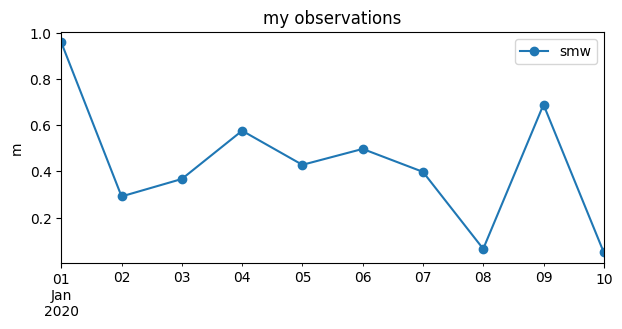
[9]:
# plot measurements
o3["value"].plot(
    figsize=(7, 3),
    label=o3.name,
    ylabel=o3.unit,
    marker="o",
    legend=True,
    title="my observations",
);
Obs types
Different Obs types have differente metadata. Groundwater observations have some extra properties screen_top, screen_bottom, ground_level, tube_top and metadata_available.
[10]:
# create a GroundwaterObs object from the Obs object
gw_obs = hpd.GroundwaterObs(
    o3,
    name="smw_pb1",
    tube_nr=1,
    screen_top=-5,
    screen_bottom=-6,
    unit="m NAP",
    ground_level=3,
    tube_top=2.95,
    metadata_available=True,
)
display(gw_obs)
hydropandas.GroundwaterObs
| smw_pb1 | |
|---|---|
| x | 1000 |
| y | 22220 |
| location | somewhere else |
| filename | |
| source | advanced imagination |
| unit | m NAP |
| tube_nr | 1 |
| screen_top | -5 |
| screen_bottom | -6 |
| ground_level | 3 |
| tube_top | 2.95 |
| metadata_available | True |
| value | |
|---|---|
| 2020-01-01 | 0.958142 |
| 2020-01-02 | 0.291446 |
| 2020-01-03 | 0.366914 |
| 2020-01-04 | 0.575771 |
| 2020-01-05 | 0.428153 |
| 2020-01-06 | 0.497021 |
| 2020-01-07 | 0.397704 |
| 2020-01-08 | 0.064448 |
| 2020-01-09 | 0.688759 |
| 2020-01-10 | 0.049285 |
Modify
Sometimes you want to change measurement values or metadata of an Obs object.
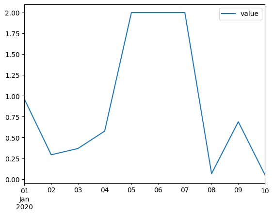
[11]:
# modify observations inplace (similar to how you modify a pandas DataFrame)
o3.loc["2020-01-05":"2020-01-7", "value"] = 2  # set value of a specific date
o3.plot()
[11]:
<Axes: >
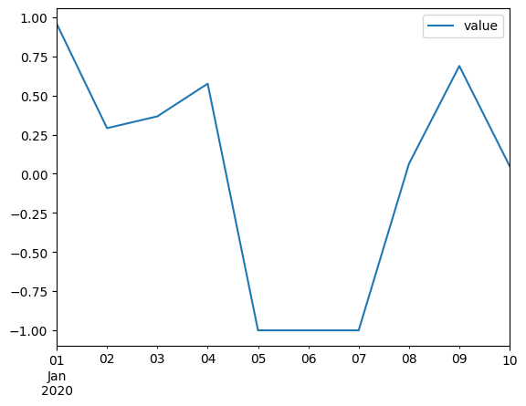
[12]:
# create a new observation with modifications
o4 = o3.copy()  # note use the copy method to create a new object
o4.loc["2020-01-05":"2020-01-7", "value"] = -1
o4.plot()
[12]:
<Axes: >
[13]:
# modify metadata by direct assignment
o4.name = "smw_modified"
o4.source = "smw"
display(o4)
hydropandas.Obs
| smw_modified | |
|---|---|
| x | 1000 |
| y | 22220 |
| location | somewhere else |
| filename | |
| source | smw |
| unit | m |
| value | |
|---|---|
| 2020-01-01 | 0.958142 |
| 2020-01-02 | 0.291446 |
| 2020-01-03 | 0.366914 |
| 2020-01-04 | 0.575771 |
| 2020-01-05 | -1.000000 |
| 2020-01-06 | -1.000000 |
| 2020-01-07 | -1.000000 |
| 2020-01-08 | 0.064448 |
| 2020-01-09 | 0.688759 |
| 2020-01-10 | 0.049285 |
Additional metadata
Sometimes you have metadata that does not match any of the default metadata names for a particular Observation type. For groundwater observations you may have the name of the company that constructed the measurement well. This additional metadata can be stored in the meta attribute as a dictionary. Below we create a GroundwaterObs object with some additional metadata.
Note that display(gw_obs) will never display the meta dictionary.
[14]:
gw_obs = hpd.GroundwaterObs(
    o3,
    name="smw_pb1",
    tube_nr=1,
    screen_top=-5,
    screen_bottom=-6,
    unit="m NAP",
    ground_level=3,
    tube_top=2.95,
    metadata_available=True,
    meta={"contractor": "GeoDrill Inc."},
)
print(gw_obs.meta)
{'contractor': 'GeoDrill Inc.'}
Read/write Obs
Observations can be read/written from/to a json, csv, excel or pickle file, see this table:
type |
write function |
read function |
Human readable |
Store metadata |
Write/read additional metadata* |
keep dtypes? |
|---|---|---|---|---|---|---|
json |
Obs.to_json |
hpd.read_json |
Yes |
Yes |
Yes |
Mostly |
csv |
Obs.to_csv |
Obs.from_csv |
Yes |
Yes |
No |
No |
pickle |
Obs.to_pickle |
Obs.from_pickle |
No |
Yes |
Yes |
Yes |
excel* |
Obs.to_excel |
pd.read_excel |
Yes (in Excel) |
No |
No |
No |
*the to_excel method is the inherited method from a pandas DataFrame. The other methods are methods adapted for hydropandas.
Json is a human readable format that can be used to store observation objects. Additional metadata is kept in the json file and it is more robust for keeping the same dtypes. At times small details, such as the index frequency, may be different between the original file and the one that is written and read to a json file.
[15]:
# write to json
gw_obs.to_json("my_gw_obs.json", indent=4)
gw_obs
[15]:
hydropandas.GroundwaterObs
| smw_pb1 | |
|---|---|
| x | 1000 |
| y | 22220 |
| location | somewhere else |
| filename | |
| source | advanced imagination |
| unit | m NAP |
| tube_nr | 1 |
| screen_top | -5 |
| screen_bottom | -6 |
| ground_level | 3 |
| tube_top | 2.95 |
| metadata_available | True |
| value | |
|---|---|
| 2020-01-01 | 0.958142 |
| 2020-01-02 | 0.291446 |
| 2020-01-03 | 0.366914 |
| 2020-01-04 | 0.575771 |
| 2020-01-05 | 2.000000 |
| 2020-01-06 | 2.000000 |
| 2020-01-07 | 2.000000 |
| 2020-01-08 | 0.064448 |
| 2020-01-09 | 0.688759 |
| 2020-01-10 | 0.049285 |
[16]:
# read from json
gw_obs_from_json = hpd.read_json("my_gw_obs.json")
gw_obs_from_json
[16]:
hydropandas.GroundwaterObs
| smw_pb1 | |
|---|---|
| x | 1000 |
| y | 22220 |
| location | somewhere else |
| filename | |
| source | advanced imagination |
| unit | m NAP |
| tube_nr | 1 |
| screen_top | -5 |
| screen_bottom | -6 |
| ground_level | 3 |
| tube_top | 2.95 |
| metadata_available | True |
| value | |
|---|---|
| 2020-01-01 | 0.958142 |
| 2020-01-02 | 0.291446 |
| 2020-01-03 | 0.366914 |
| 2020-01-04 | 0.575771 |
| 2020-01-05 | 2.000000 |
| 2020-01-06 | 2.000000 |
| 2020-01-07 | 2.000000 |
| 2020-01-08 | 0.064448 |
| 2020-01-09 | 0.688759 |
| 2020-01-10 | 0.049285 |
[17]:
print("index frequency original:", gw_obs.index.freq)
print("index frequency from json:", gw_obs_from_json.index.freq)
index frequency original: <Day>
index frequency from json: None
When Obs object are written and read from a csv file: 1. The datatypes may have changed 2. The additional metadata in the .meta attribute is lost.
[18]:
# save the groundwater observations to a csv file
gw_obs.to_csv("my_gw_obs.csv")
WARNING:hydropandas.observation.to_csv:additional metadata of observation smw_pb1 not written to csv, consider using the to_json method to keep the metadata
[19]:
# read the groundwater observations from a csv file
gw_obs_from_csv = hpd.GroundwaterObs.from_csv("my_gw_obs.csv")
[20]:
# 1. datatypes changed
print("datatype of gw_obs.screen_top:", type(gw_obs.screen_top))
print("datatype of gw_obs_from_csv.screen_top:", type(gw_obs_from_csv.screen_top))

# 2. additional metadata is not saved in the csv file
print(f"\nadditional metadata: {gw_obs.meta=}")
print(f"additional metadata: {gw_obs_from_csv.meta=}")
datatype of gw_obs.screen_top: <class 'int'>
datatype of gw_obs_from_csv.screen_top: <class 'float'>

additional metadata: gw_obs.meta={'contractor': 'GeoDrill Inc.'}
additional metadata: gw_obs_from_csv.meta={}
Pickle files are binary and not readable for humans. They are very fast to write/read and return an exact copy of the original file. Pickle files are not very useful for long-term storage because they:
are only readable in Python
are not stable across Python and package versions.
contain references to exact class and module paths
[21]:
# save the object to a pickle file
gw_obs.to_pickle("my_gw_obs.pklz")
[22]:
# read the object from a pickle file
gw_obs2 = hpd.read_pickle("my_gw_obs.pklz")
[23]:
gw_obs2.equals(gw_obs) # check if the two objects are equal
[23]:
True
ObsCollection
An ObsCollection is a structured way to manage and analyse multiple time series of hydrological observations. It serves as a container for multiple Obs objects, which represent individual time series of measurements, such as groundwater levels, precipitation, or water quality.
Each row in an ObsCollection contains metadata (e.g., location, station name) and a corresponding Obs object holding the time series data. This structure allows for easy comparison, filtering, and statistical analysis across multiple observation sites.
[24]:
# create an empty ObsCollection
oc = hpd.ObsCollection()
print(oc)
Empty ObsCollection
Columns: []
Index: []
[25]:
# create an ObsCollection with a single Obs object
oc = hpd.ObsCollection(o3)
oc
[25]:
| x | y | location | filename | source | unit | obs | |
|---|---|---|---|---|---|---|---|
| name | |||||||
| smw | 1000 | 22220 | somewhere else | advanced imagination | m | Obs smw -----metadata------ name : smw x : 10... |
[26]:
# create an ObsCollection with multiple Obs objects
oc = hpd.ObsCollection([o1, o2, o3])
oc
[26]:
| x | y | location | filename | source | unit | obs | |
|---|---|---|---|---|---|---|---|
| name | |||||||
| my empty obs | NaN | NaN | Obs my empty obs -----metadata------ name : my... | ||||
| my_observation | 10.0 | 20.0 | somewhere | unknown | imagination | m | Obs my_observation -----metadata------ name : ... |
| smw | 1000.0 | 22220.0 | somewhere else | advanced imagination | m | Obs smw -----metadata------ name : smw x : 10... |
ObsCollection metadata
Access the metadata using the standard DataFrame methods.
[27]:
print(f"the x coordinate of observation 2 is: {oc.loc['my_observation', 'x']}")
print(f"the location of observation 3 is: {oc.loc['smw', 'location']}")
the x coordinate of observation 2 is: 10.0
the location of observation 3 is: somewhere else
ObsCollection observations
Access the Obs objects from the collection
[28]:
# using the loc method
o3_1 = oc.loc["smw", "obs"]

# using the get_obs method with the name of the observation
o3_2 = oc.get_obs("smw")

# using the get_obs method with the location (only works if the location is unique)
o3_3 = oc.get_obs(location="somewhere else")

# check if the three objects are the same
id(o3_1) == id(o3_2) == id(o3_3)
[28]:
True
Slice ObsCollection
Filter and slice ObsCollections
[29]:
oc.loc[oc["y"] > 10] # Selection based on the y coordinate
[29]:
| x | y | location | filename | source | unit | obs | |
|---|---|---|---|---|---|---|---|
| name | |||||||
| my_observation | 10.0 | 20.0 | somewhere | unknown | imagination | m | Obs my_observation -----metadata------ name : ... |
| smw | 1000.0 | 22220.0 | somewhere else | advanced imagination | m | Obs smw -----metadata------ name : smw x : 10... |
[30]:
oc.loc[oc["source"].str.contains("advanced")] # Selection based on the location
[30]:
| x | y | location | filename | source | unit | obs | |
|---|---|---|---|---|---|---|---|
| name | |||||||
| smw | 1000.0 | 22220.0 | somewhere else | advanced imagination | m | Obs smw -----metadata------ name : smw x : 10... |
Modify ObsCollections
Below are some examples to modify ObsCollections. More details on merging observations and ObsCollections are available here.
remove an observation
add an observation
modify metadata of an observation
update the timeseries of an observation with new measurements
merge observations
Remove an observation from an ObsCollection using drop.
[31]:
# remove an observation
oc.drop("my_observation", inplace=True)
Add an observation from an ObsCollection using add_observation.
Note: Adding an observation using oc.loc[<name>,'obs'] = o does not work and results in an empty ‘obs’ column
[32]:
# add an observation
oc.add_observation(o2, inplace=True)
oc
INFO:hydropandas.obs_collection.add_observation:adding my_observation to collection
[32]:
| x | y | location | filename | source | unit | obs | |
|---|---|---|---|---|---|---|---|
| name | |||||||
| my empty obs | NaN | NaN | Obs my empty obs -----metadata------ name : my... | ||||
| smw | 1000.0 | 22220.0 | somewhere else | advanced imagination | m | Obs smw -----metadata------ name : smw x : 10... | |
| my_observation | 10.0 | 20.0 | somewhere | unknown | imagination | m | Obs my_observation -----metadata------ name : ... |
[33]:
# Do not add observations using loc!
oc_copy = oc.copy(deep=True)
oc_copy.loc["new_obs", "obs"] = gw_obs
oc_copy
[33]:
| x | y | location | filename | source | unit | obs | |
|---|---|---|---|---|---|---|---|
| name | |||||||
| my empty obs | NaN | NaN | Obs my empty obs -----metadata------ name : my... | ||||
| smw | 1000.0 | 22220.0 | somewhere else | advanced imagination | m | Obs smw -----metadata------ name : smw x : 10... | |
| my_observation | 10.0 | 20.0 | somewhere | unknown | imagination | m | Obs my_observation -----metadata------ name : ... |
| new_obs | NaN | NaN | NaN | NaN | NaN | NaN | NaN |
Use the set_metadata_value on the ObsCollection to modify metadata.
Note: Metadata of a single observation is stored in two places: in the ObsCollection DataFrame and in the attribute of the Observation object. set_metadata_value will modify both which is preferred over setting the value only in the ObsCollection dataframe or only in the Observation attribute. The latter two will result in an inconsistent ObsCollection.
[34]:
# modify metadata of an observation
oc.set_metadata_value("my_observation", "x", 1815)
oc.set_metadata_value("my_observation", "y", 2025)
print(oc._is_consistent())  # check if the ObsCollection is consistent
True
[35]:
# Do not use this way to modify metadata!
oc_copy = oc.copy(deep=True)
oc_copy.loc["smw", "x"] = 100
oc_copy._is_consistent()  # check if the ObsCollection is consistent
WARNING:hydropandas.obs_collection._is_consistent:observation collection '' not consistent because of metadata value 'x' of observation 'smw'
[35]:
False
There are several ways to update an observation with new measurements. The most robust is using: 1. Make a copy of the observation from the collection 2. Remove the observation from the collection 3. Modify the Obs object according to your wishes 4. Add the observation back to the collection
[36]:
# New measurements
new_measurements = pd.DataFrame(
    index=pd.date_range(start="2020-01-11", periods=10, freq="D"),
    data={"value": np.random.rand(10)},
)
new_o = hpd.Obs(
    new_measurements,
    name="smw",
    x=1000,
    y=22220,
    location="somewhere else",
    source="advanced imagination",
    unit="m",
)

# 1. create a copy of an observation
o = oc.loc["smw", "obs"].copy()

# 2. delete observation from collection
oc.drop(o.name, inplace=True)

# 3. Update existing observation with new measurements
o_updated = o.merge_observation(new_o)

# 4. add modified observation to collection
oc.add_observation(o_updated, inplace=True)
oc
INFO:hydropandas.observation._merge_timeseries:right observation has a different time series
INFO:hydropandas.observation._merge_timeseries:merge time series
INFO:hydropandas.observation.merge_metadata:left and right observation have the same metadata
INFO:hydropandas.obs_collection.add_observation:adding smw to collection
[36]:
| x | y | location | filename | source | unit | obs | |
|---|---|---|---|---|---|---|---|
| name | |||||||
| my empty obs | NaN | NaN | Obs my empty obs -----metadata------ name : my... | ||||
| my_observation | 1815.0 | 2025.0 | somewhere | unknown | imagination | m | Obs my_observation -----metadata------ name : ... |
| smw | 1000.0 | 22220.0 | somewhere else | advanced imagination | m | Obs smw -----metadata------ name : smw x : 10... |
Sometimes you may be able to modify the time series directly. Below we show a way using chained assignment and a two-step plan. This way of modifying a time series does not always work so we encourage to use the more robust method shown above.
[37]:
# modify the timeseries of an observation

# 1 chained assignment
oc.loc["smw", "obs"].loc["2020-1-7":"2020-1-9", "value"] = 42
display(oc.loc["smw", "obs"])

# 2 two-step
o = oc.loc["smw", "obs"]
o.loc["2020-1-7":"2020-1-9", "value"] = 21
display(oc.loc["smw", "obs"])
hydropandas.Obs
| smw | |
|---|---|
| x | 1000 |
| y | 22220 |
| location | somewhere else |
| filename | |
| source | advanced imagination |
| unit | m |
| value | |
|---|---|
| 2020-01-01 | 0.958142 |
| 2020-01-02 | 0.291446 |
| 2020-01-03 | 0.366914 |
| 2020-01-04 | 0.575771 |
| 2020-01-05 | 2.000000 |
| 2020-01-06 | 2.000000 |
| 2020-01-07 | 42.000000 |
| 2020-01-08 | 42.000000 |
| 2020-01-09 | 42.000000 |
| 2020-01-10 | 0.049285 |
| 2020-01-11 | 0.435199 |
| 2020-01-12 | 0.220779 |
| 2020-01-13 | 0.143853 |
| 2020-01-14 | 0.043459 |
| 2020-01-15 | 0.137335 |
| 2020-01-16 | 0.388173 |
| 2020-01-17 | 0.449079 |
| 2020-01-18 | 0.021230 |
| 2020-01-19 | 0.208231 |
| 2020-01-20 | 0.735086 |
hydropandas.Obs
| smw | |
|---|---|
| x | 1000 |
| y | 22220 |
| location | somewhere else |
| filename | |
| source | advanced imagination |
| unit | m |
| value | |
|---|---|
| 2020-01-01 | 0.958142 |
| 2020-01-02 | 0.291446 |
| 2020-01-03 | 0.366914 |
| 2020-01-04 | 0.575771 |
| 2020-01-05 | 2.000000 |
| 2020-01-06 | 2.000000 |
| 2020-01-07 | 21.000000 |
| 2020-01-08 | 21.000000 |
| 2020-01-09 | 21.000000 |
| 2020-01-10 | 0.049285 |
| 2020-01-11 | 0.435199 |
| 2020-01-12 | 0.220779 |
| 2020-01-13 | 0.143853 |
| 2020-01-14 | 0.043459 |
| 2020-01-15 | 0.137335 |
| 2020-01-16 | 0.388173 |
| 2020-01-17 | 0.449079 |
| 2020-01-18 | 0.021230 |
| 2020-01-19 | 0.208231 |
| 2020-01-20 | 0.735086 |
There are several ways to merge observations. For example if you want to overwrite measurements in an ObsCollection with new data. Use the add_observation method to merge new measurements to an existing observation.
More options for merging observations in the example notebook 04_merging_observations.
[38]:
# New observation with new measurements
measurement_correction = pd.DataFrame(
    index=pd.date_range(start="2020-01-11", periods=10, freq="D"),
    data={"value": np.random.rand(10)},
)
corr_o = hpd.Obs(
    measurement_correction,
    name="smw",
    x=1000,
    y=22220,
    location="somewhere else",
    source="advanced imagination",
    unit="m",
)
[39]:
# update existing observation with new measurements
oc.add_observation(corr_o, inplace=True, overlap="use_right")

# show merged observation
oc.loc["smw", "obs"]
INFO:hydropandas.obs_collection.add_observation:observation name smw already in collection, merging observations
INFO:hydropandas.observation._merge_timeseries:right observation has a different time series
INFO:hydropandas.observation._merge_timeseries:merge time series
WARNING:hydropandas.observation._merge_timeseries:timeseries of observation smw overlap with different values
INFO:hydropandas.observation.merge_metadata:left and right observation have the same metadata
[39]:
hydropandas.Obs
| smw | |
|---|---|
| x | 1000 |
| y | 22220 |
| location | somewhere else |
| filename | |
| source | advanced imagination |
| unit | m |
| value | |
|---|---|
| 2020-01-01 | 0.958142 |
| 2020-01-02 | 0.291446 |
| 2020-01-03 | 0.366914 |
| 2020-01-04 | 0.575771 |
| 2020-01-05 | 2.000000 |
| 2020-01-06 | 2.000000 |
| 2020-01-07 | 21.000000 |
| 2020-01-08 | 21.000000 |
| 2020-01-09 | 21.000000 |
| 2020-01-10 | 0.049285 |
| 2020-01-11 | 0.807402 |
| 2020-01-12 | 0.326016 |
| 2020-01-13 | 0.091335 |
| 2020-01-14 | 0.907015 |
| 2020-01-15 | 0.655285 |
| 2020-01-16 | 0.195266 |
| 2020-01-17 | 0.089207 |
| 2020-01-18 | 0.857873 |
| 2020-01-19 | 0.793008 |
| 2020-01-20 | 0.324842 |
ObsCollection additional metadata
Additional metadata is not shown by default in an ObsCollection. It can be added manually by calling the add_meta_to_df method. By default all metadata is added but you can also specify a key from the meta dictionary to add.
[40]:
# create an Obs object with additional metadata
o2_with_meta = hpd.Obs(
    name="my_observation",
    x=10,
    y=20,
    location="somewhere",
    filename="unknown",
    source="imagination",
    unit="m",
    meta={"owner": "me", "project": "hydropandas"},
)

# create an ObsCollection with multiple Obs objects, one of them with additional metadata
oc = hpd.ObsCollection([o1, o2_with_meta, o3])

# metadata is not shown by default
oc
[40]:
| x | y | location | filename | source | unit | obs | |
|---|---|---|---|---|---|---|---|
| name | |||||||
| my empty obs | NaN | NaN | Obs my empty obs -----metadata------ name : my... | ||||
| my_observation | 10.0 | 20.0 | somewhere | unknown | imagination | m | Obs my_observation -----metadata------ name : ... |
| smw | 1000.0 | 22220.0 | somewhere else | advanced imagination | m | Obs smw -----metadata------ name : smw x : 10... |
[41]:
# add metadata to the dataframe to show it
oc_with_meta = oc.add_meta_to_df()
oc_with_meta
[41]:
| x | y | location | filename | source | unit | obs | owner | project | |
|---|---|---|---|---|---|---|---|---|---|
| name | |||||||||
| my empty obs | NaN | NaN | Obs my empty obs -----metadata------ name : my... | None | None | ||||
| my_observation | 10.0 | 20.0 | somewhere | unknown | imagination | m | Obs my_observation -----metadata------ name : ... | me | hydropandas |
| smw | 1000.0 | 22220.0 | somewhere else | advanced imagination | m | Obs smw -----metadata------ name : smw x : 10... | None | None |
Read/write ObsCollection
There are several options to read/write an ObsCollection from/to a file. The table below gives a broad overview on the options
type |
write function |
read function |
Human readable |
Write/read additional metadata* |
keep dtypes? |
|---|---|---|---|---|---|
json |
ObsCollection.to_json |
hpd.read_json |
Yes |
Yes |
Mostly |
csv |
ObsCollection.to_csv |
hpd.read_csv |
Yes |
No |
No |
excel |
ObsCollection.to_excel |
hpd.read_excel |
Yes (via excel) |
Only if exposed in oc** |
No |
pickle |
ObsCollection.to_pickle |
hpd.read_pickle |
No |
Yes |
Yes |
Writing to and reading from an excel, csv or json file slightly alters the properties of the ObsCollection, just like writing and reading a DataFrame to these file types would do. Reading/writing a pickle does not change anything.
** Additional metadata is only written and read if it was added to the ObsCollection using the add_meta_to_df method. More info on additional metadata here.
[42]:
path = "my_obs_collection.json"
oc_with_meta.to_json(path, indent=4)
oc_with_meta
[42]:
| x | y | location | filename | source | unit | obs | owner | project | |
|---|---|---|---|---|---|---|---|---|---|
| name | |||||||||
| my empty obs | NaN | NaN | Obs my empty obs -----metadata------ name : my... | None | None | ||||
| my_observation | 10.0 | 20.0 | somewhere | unknown | imagination | m | Obs my_observation -----metadata------ name : ... | me | hydropandas |
| smw | 1000.0 | 22220.0 | somewhere else | advanced imagination | m | Obs smw -----metadata------ name : smw x : 10... | None | None |
[43]:
oc_from_json = hpd.read_json(path)
oc_from_json
[43]:
| x | y | location | filename | source | unit | owner | project | obs | |
|---|---|---|---|---|---|---|---|---|---|
| my empty obs | NaN | NaN | None | None | Obs my empty obs -----metadata------ name : my... | ||||
| my_observation | 10.0 | 20.0 | somewhere | unknown | imagination | m | me | hydropandas | Obs my_observation -----metadata------ name : ... |
| smw | 1000.0 | 22220.0 | somewhere else | advanced imagination | m | None | None | Obs smw -----metadata------ name : smw x : 10... |
[44]:
csvdir = "my_obs_collection"
oc_with_meta.to_csv(csvdir)
oc_with_meta
INFO:hydropandas.obs_collection.to_csv:writing 3 observations to my_obs_collection
WARNING:hydropandas.observation.to_csv:additional metadata of observation my_observation not written to csv, consider using the to_json method to keep the metadata
[44]:
| x | y | location | filename | source | unit | obs | owner | project | |
|---|---|---|---|---|---|---|---|---|---|
| name | |||||||||
| my empty obs | NaN | NaN | Obs my empty obs -----metadata------ name : my... | None | None | ||||
| my_observation | 10.0 | 20.0 | somewhere | unknown | imagination | m | Obs my_observation -----metadata------ name : ... | me | hydropandas |
| smw | 1000.0 | 22220.0 | somewhere else | advanced imagination | m | Obs smw -----metadata------ name : smw x : 10... | None | None |
[45]:
oc_from_csv = hpd.read_csv(csvdir)  # read the ObsCollection from the csv files
oc_from_csv
[45]:
| x | y | location | filename | source | unit | obs | |
|---|---|---|---|---|---|---|---|
| name | |||||||
| my_observation | 10.0 | 20.0 | somewhere | unknown | imagination | m | Obs my_observation -----metadata------ name : ... |
| smw | 1000.0 | 22220.0 | somewhere else | advanced imagination | m | Obs smw -----metadata------ name : smw x : 10... | |
| my empty obs | NaN | NaN | Obs my empty obs -----metadata------ name : my... |
[46]:
oc_with_meta.to_excel("my_obs_collection.xlsx") # write to excel
[47]:
# read excel file
oc_from_excel = hpd.read_excel("my_obs_collection.xlsx")
oc_from_excel
[47]:
| x | y | location | filename | source | unit | owner | project | obs | |
|---|---|---|---|---|---|---|---|---|---|
| name | |||||||||
| my empty obs | NaN | NaN | NaN | NaN | NaN | NaN | NaN | NaN | Obs my empty obs -----metadata------ name : my... |
| my_observation | 10.0 | 20.0 | somewhere | unknown | imagination | m | me | hydropandas | Obs my_observation -----metadata------ name : ... |
| smw | 1000.0 | 22220.0 | somewhere else | NaN | advanced imagination | m | NaN | NaN | Obs smw -----metadata------ name : smw x : 10... |
[48]:
oc_with_meta.to_pickle("my_obs_collection.pklz") # write to pickle
[49]:
# read pickle
oc_from_pickle = hpd.read_pickle("my_obs_collection.pklz")
oc_from_pickle
[49]:
| x | y | location | filename | source | unit | obs | owner | project | |
|---|---|---|---|---|---|---|---|---|---|
| name | |||||||||
| my empty obs | NaN | NaN | Obs my empty obs -----metadata------ name : my... | None | None | ||||
| my_observation | 10.0 | 20.0 | somewhere | unknown | imagination | m | Obs my_observation -----metadata------ name : ... | me | hydropandas |
| smw | 1000.0 | 22220.0 | somewhere else | advanced imagination | m | Obs smw -----metadata------ name : smw x : 10... | None | None |
Extensions
To enhance the functionality of an ObsCollection, HydroPandas provides several extensions that add specialized methods for visualization, spatial analysis, and data processing. Some key extensions include:
Plot Extension (ObsCollection.plot): Built-in plotting capabilities for visualizing time series data. Users can generate time series plots for individual or multiple observations, histograms, and other graphical representations to analyze trends and patterns in hydrological data.
Geo Extension (ObsCollection.geo): Spatial analysis by integrating with geopandas. It allows users to obtain the extent of an ObsCollection, convert to another coordinate reference system and find nearby geometries.
Groundwater Obs (ObsCollection.gwobs): Analyse and process groundwater observations. Users can find the REGIS layer of each tube and set the tube number based on the screen depth.
Statistics (ObsCollection.stats): Statistical analysis of the observations. Users can obtain the number of consecutive years with more than 10 observations or find seasonal minimum and maximum values.
[50]:
oc.stats.get_first_last_obs_date() # get the first and last observation date using the stats extension
[50]:
| date_first_measurement | date_last_measurement | |
|---|---|---|
| name | ||
| my empty obs | NaT | NaT |
| my_observation | NaT | NaT |
| smw | 2020-01-01 | 2020-01-10 |
[51]:
oc.geo.get_extent() # get the extent of the observations using the geo extension
[51]:
(np.float64(10.0), np.float64(1000.0), np.float64(20.0), np.float64(22220.0))