Hydropandas and Pastas

This notebook demonstrates how hydropandas can be used to build Pastas Models. Pastas is a Python package that can be used to simulate and analyze groundwater time series. One of the biggest challenges when making a Pastas Model is to find a valid dataset. The Hydropandas packages can be used to obtain such a dataset. This notebook shows how to build a simple pastas model from Dutch data.

Groundwater observations
Meteo observations
Pastas model
Surface water observations
Pastastore

[1]:

import pastas as ps

import hydropandas as hpd

ps.set_log_level("ERROR")
hpd.util.get_color_logger("INFO")

print(hpd.__version__)
print(ps.__version__)

0.18.1
1.13.2

Groundwater observations 

First we read the groundwater level observation using the from_dino function of a GroundwaterObs object. The code below reads the groundwater level timeseries from a csv file in the data directory.

[2]:

gw_levels = hpd.GroundwaterObs.from_dino(r"data/B49F0555001_1.csv")

INFO:hydropandas.io.dino.read_dino_groundwater_csv:reading -> B49F0555001_1

Note that gw_levels is a GroundwaterObs object. This is basically a pandas DataFrame with additional methods and attributes related to groundwater level observations. We can print gw_levels to see all of its properties.

[3]:

print(gw_levels)

GroundwaterObs B49F0555-001
-----metadata------
name : B49F0555-001
x : 94532.0
y : 399958.0
location : B49F0555
filename : B49F0555001_1
source : dino
unit : m NAP
tube_nr : 1.0
screen_top : -0.75
screen_bottom : -1.75
ground_level : -0.61
tube_top : -0.15
metadata_available : True

-----time series------
            stand_m_tov_nap   locatie  filternummer  stand_cm_tov_mp  \
peildatum
2003-02-14            -0.64  B49F0555             1             49.0
2003-02-26            -0.71  B49F0555             1             56.0
2003-03-14            -0.81  B49F0555             1             66.0
2003-03-28            -0.92  B49F0555             1             77.0
2003-04-14            -0.81  B49F0555             1             66.0
...                     ...       ...           ...              ...
2013-10-26            -0.71  B49F0555             1             56.0
2013-10-27            -0.72  B49F0555             1             57.0
2013-10-28            -0.71  B49F0555             1             56.0
2013-10-29            -0.67  B49F0555             1             52.0
2013-10-30            -0.66  B49F0555             1             51.0

            stand_cm_tov_mv  stand_cm_tov_nap bijzonderheid  opmerking
peildatum
2003-02-14              3.0             -64.0           NaN        NaN
2003-02-26             10.0             -71.0           NaN        NaN
2003-03-14             20.0             -81.0           NaN        NaN
2003-03-28             31.0             -92.0           NaN        NaN
2003-04-14             20.0             -81.0           NaN        NaN
...                     ...               ...           ...        ...
2013-10-26             10.0             -71.0           NaN        NaN
2013-10-27             11.0             -72.0           NaN        NaN
2013-10-28             10.0             -71.0           NaN        NaN
2013-10-29              6.0             -67.0           NaN        NaN
2013-10-30              5.0             -66.0           NaN        NaN

[2241 rows x 8 columns]

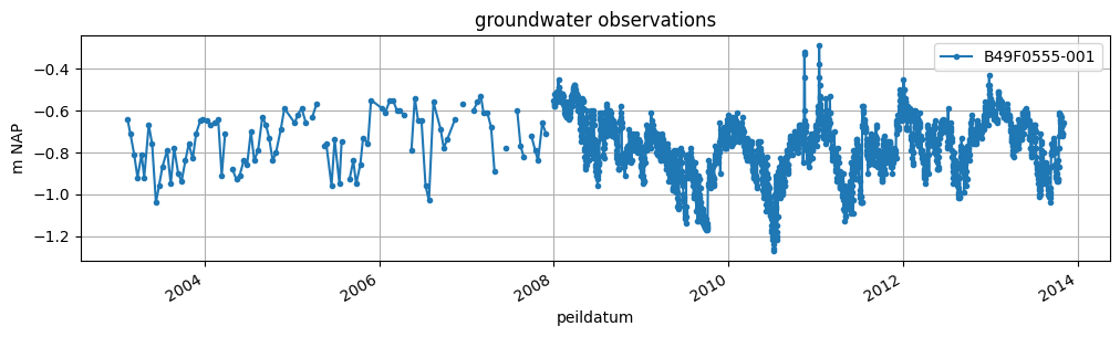
The GroundwaterObs object comes with its own plot methods, to quickly visualize the data:

[4]:

ax = gw_levels["stand_m_tov_nap"].plot(
    figsize=(12, 3),
    marker=".",
    grid=True,
    label=gw_levels.name,
    legend=True,
    ylabel="m NAP",
    title="groundwater observations",
)

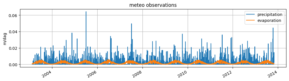
../_images/examples_03_hydropandas_and_pastas_7_0.png

Meteo observations 

We can obtain evaporation and precipitation data from the knmi using the from_knmi_nearest_xy method in hydropandas. For a given set of (x,y) coordinates it will find the closest KNMI meteostation and download the data. If there are missing measurements they are filled automatically using the value of a nearby station.

[5]:

evaporation = hpd.EvaporationObs.from_knmi(
    xy=(gw_levels.x, gw_levels.y),
    meteo_var="EV24",
    start=gw_levels.index[0],
    end=gw_levels.index[-1],
    fill_missing_obs=True,
)
precipitation = hpd.PrecipitationObs.from_knmi(
    xy=(gw_levels.x, gw_levels.y),
    start=gw_levels.index[0],
    end=gw_levels.index[-1],
    fill_missing_obs=True,
)

INFO:hydropandas.io.knmi.get_knmi_obs:get KNMI data from station nearest to coordinates (94532.0, 399958.0) and meteovariable EV24
INFO:hydropandas.io.knmi.get_knmi_obs:get KNMI data from station nearest to coordinates (94532.0, 399958.0) and meteovariable RH
INFO:hydropandas.io.knmi.fill_missing_measurements:station 340 has no measurements between 2003-02-14 00:00:00 and 2013-10-30 00:00:00 trying to get measurements from nearest station -> 319

[6]:

ax = precipitation["RH"].plot(label="precipitation", legend=True, figsize=(12, 3))
evaporation["EV24"].plot(
    ax=ax,
    label="evaporation",
    legend=True,
    grid=True,
    ylabel="m/dag",
    title="meteo observations",
)

[6]:

<Axes: title={'center': 'meteo observations'}, ylabel='m/dag'>

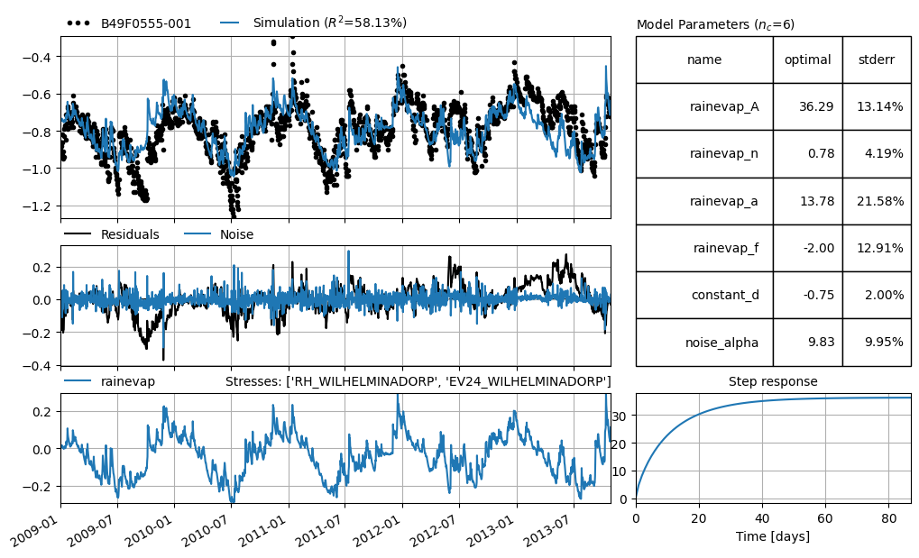
../_images/examples_03_hydropandas_and_pastas_10_1.png

Pastas model 

Now that we have groundwater observations and meteo data we can create a Pastas model.

[7]:

ml = ps.Model(gw_levels["stand_m_tov_nap"], name=gw_levels.name)

# Add the recharge data as explanatory variable
ts1 = ps.RechargeModel(
    precipitation["RH"].resample("D").first(),
    evaporation["EV24"].resample("D").first(),
    ps.Gamma(),
    name="rainevap",
    settings=("prec", "evap"),
)

ml.add_stressmodel(ts1)

ml.solve(tmin="2009")

Fit report B49F0555-001             Fit Statistics
==================================================
nfev     18                     EVP          73.45
nobs     1764                   R2            0.73
noise    False                  RMSE          0.07
tmin     2009-01-01 00:00:00    AICc      -9270.98
tmax     2013-10-30 00:00:00    BIC       -9243.64
freq     D                      Obj           4.58
freq_obs None                   ___
warmup   3650 days 00:00:00     Interp.         No
solver   LeastSquares           weights        Yes

Parameters (5 optimized)
==================================================
                optimal     initial  vary
rainevap_A  1193.920428  196.769293  True
rainevap_n     0.568433    1.000000  True
rainevap_a  9999.999998   10.000000  True
rainevap_f    -0.976022   -1.000000  True
constant_d    -1.233222   -0.774436  True

Warnings! (3)
==================================================
Parameter 'rainevap_a' on upper bound: 1.00e+04
Response tmax for 'rainevap' > than calibration period.
Response tmax for 'rainevap' > than warmup period.

[8]:

ml.plots.results(figsize=(10, 6))

[8]:

[<Axes: xlabel='peildatum', ylabel='Head'>,
 <Axes: >,
 <Axes: title={'right': "Stresses: ['RH', 'EV24']"}, ylabel='Rise'>,
 <Axes: title={'center': 'Step response'}>,
 <Axes: title={'left': 'Model parameters ($n_c$=5)'}>]

../_images/examples_03_hydropandas_and_pastas_13_1.png

Surface water observations 

Our model is not always able to simulate the groundwater level accurately. Maybe it will improve if we add surface water observations. The code below is used to read the surface water level timeseries from a csv file in the data directory.

[9]:

river_levels = hpd.WaterlvlObs.from_dino(r"data/P43H0001.csv")

INFO:hydropandas.io.dino.read_dino_waterlvl_csv:reading -> P43H0001

We can plot the data together with the groundwater levels.

[10]:

ax = gw_levels["stand_m_tov_nap"].plot(
    figsize=(12, 3),
    label=gw_levels.name,
    ylabel="m NAP",
    title="observations",
    legend=True,
)
river_levels["stand_m_tov_nap"].plot(
    ax=ax, grid=True, label=river_levels.name, legend=True
)

[10]:

<Axes: title={'center': 'observations'}, xlabel='peildatum', ylabel='m NAP'>

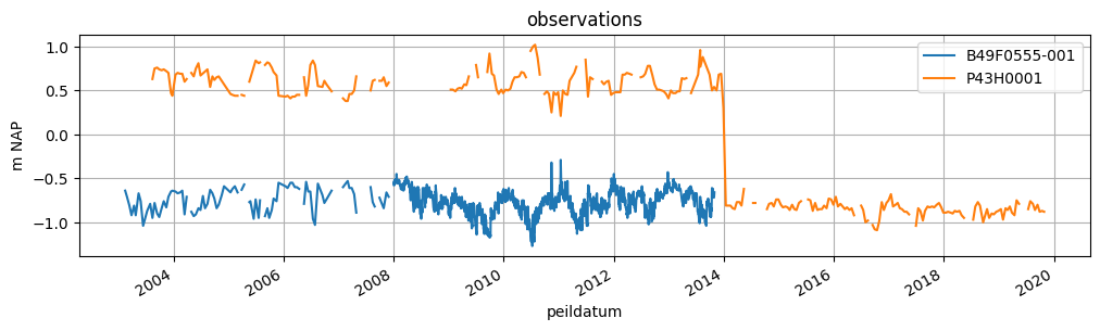
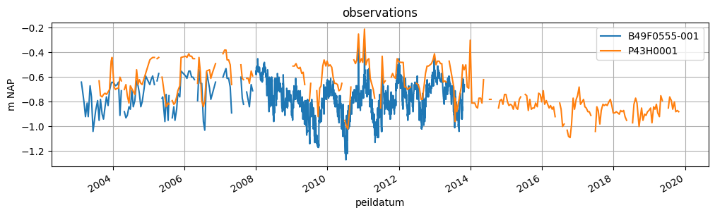
../_images/examples_03_hydropandas_and_pastas_17_1.png

As can be observed in the plot above, there is a downward shift in the surface water levels at the end of 2014. Clearly something went wrong with the registration of the river levels. We assume that the negative values from the end of 2014 onwards are correct. The positive values were registered incorrectly (missing a minus sign). We fix the timeseries by updating the ‘stand_m_tov_nap’ column of the WaterlvlObs object named river_levels.

[11]:

river_levels["stand_m_tov_nap"] = river_levels["stand_m_tov_nap"].abs() * -1

Now we plot the timeseries again, to see if the applied fix looks reasonable.

[12]:

ax = gw_levels["stand_m_tov_nap"].plot(
    figsize=(12, 3),
    label=gw_levels.name,
    ylabel="m NAP",
    title="observations",
    legend=True,
)
river_levels["stand_m_tov_nap"].plot(
    ax=ax, grid=True, label=river_levels.name, legend=True
)

[12]:

<Axes: title={'center': 'observations'}, xlabel='peildatum', ylabel='m NAP'>

../_images/examples_03_hydropandas_and_pastas_21_1.png

Now we add the river levels as an external stress in the pastas model.

[13]:

w = ps.StressModel(
    river_levels["stand_m_tov_nap"].resample("D").first(),
    rfunc=ps.One(),
    name="waterlevel",
    settings="waterlevel",
)
ml.add_stressmodel(w)
ml.solve(tmin="2009")

ml.plots.results(figsize=(10, 6))

Fit report B49F0555-001             Fit Statistics
==================================================
nfev     17                     EVP          77.90
nobs     1764                   R2            0.78
noise    False                  RMSE          0.07
tmin     2009-01-01 00:00:00    AICc      -9592.10
tmax     2013-10-30 00:00:00    BIC       -9559.30
freq     D                      Obj           3.81
freq_obs None                   ___
warmup   3650 days 00:00:00     Interp.         No
solver   LeastSquares           weights        Yes

Parameters (6 optimized)
==================================================
                   optimal     initial  vary
rainevap_A      950.557914  196.769293  True
rainevap_n        0.575904    1.000000  True
rainevap_a    10000.000000   10.000000  True
rainevap_f       -0.837625   -1.000000  True
waterlevel_d      0.325266    0.161028  True
constant_d       -1.073519   -0.774436  True

Warnings! (3)
==================================================
Parameter 'rainevap_a' on upper bound: 1.00e+04
Response tmax for 'rainevap' > than calibration period.
Response tmax for 'rainevap' > than warmup period.

[13]:

[<Axes: xlabel='peildatum', ylabel='Head'>,
 <Axes: >,
 <Axes: title={'right': "Stresses: ['RH', 'EV24']"}, ylabel='Rise'>,
 <Axes: title={'center': 'Step response'}>,
 <Axes: title={'right': "Stresses: ['stand_m_tov_nap']"}, ylabel='Rise'>,
 <Axes: title={'center': 'Step response'}>,
 <Axes: title={'left': 'Model parameters ($n_c$=6)'}>]

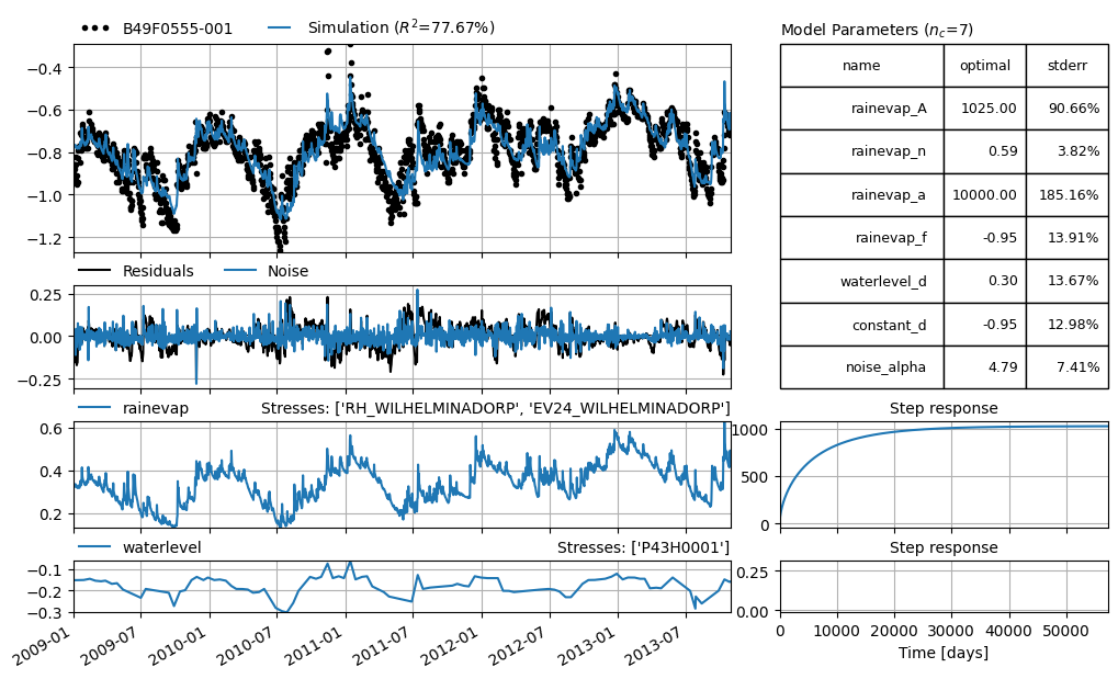
../_images/examples_03_hydropandas_and_pastas_23_2.png

We can see that the evp has increased when we’ve added the water level stress, does this mean that the model improved? Please have a look at the pastas documentation for more information on this subject.

Pastastore 

We can also use the hydropandas package to create a PastaStore with multiple observations. A Pastastore is a combination of observations, stresses and pastas time series models. More information on the Pastastore can be found here.

Groundwater observations

First we read multiple observations from a directory with dino groundwater measurements. We store them in an ObsCollection object named oc_dino.

[14]:

extent = [117850, 117980, 439550, 439700]  # Schoonhoven zuid-west
dinozip = "data/dino.zip"
oc_dino = hpd.read_dino(
    dirname=dinozip, subdir="Grondwaterstanden_Put", suffix="1.csv", keep_all_obs=False
)
oc_dino = oc_dino.loc[
    ["B58A0092-004", "B58A0092-005", "B58A0102-001", "B58A0167-001", "B58A0212-001"]
]
oc_dino

INFO:hydropandas.io.dino.read_dino_groundwater_csv:reading -> Grondwaterstanden_Put/B02H0092001_1.csv
WARNING:hydropandas.io.dino.read_dino_groundwater_csv:no NAP measurements available -> Grondwaterstanden_Put/B02H0092001_1.csv
INFO:hydropandas.io.dino.read_dino_groundwater_csv:reading -> Grondwaterstanden_Put/B02H1007001_1.csv
WARNING:hydropandas.io.dino.read_dino_groundwater_csv:no NAP measurements available -> Grondwaterstanden_Put/B02H1007001_1.csv
INFO:hydropandas.io.dino.read_dino_groundwater_csv:reading -> Grondwaterstanden_Put/B04D0032002_1.csv
WARNING:hydropandas.io.dino.read_dino_groundwater_csv:could not read metadata -> Grondwaterstanden_Put/B04D0032002_1.csv
WARNING:hydropandas.io.dino.read_dino_groundwater_csv:no NAP measurements available -> Grondwaterstanden_Put/B04D0032002_1.csv
INFO:root.get_dino_obs:not added to collection -> Grondwaterstanden_Put/B04D0032002_1.csv
INFO:hydropandas.io.dino.read_dino_groundwater_csv:reading -> Grondwaterstanden_Put/B27D0260001_1.csv
WARNING:hydropandas.io.dino.read_dino_groundwater_csv:could not read metadata -> Grondwaterstanden_Put/B27D0260001_1.csv
WARNING:hydropandas.io.dino.read_dino_groundwater_csv:no NAP measurements available -> Grondwaterstanden_Put/B27D0260001_1.csv
INFO:root.get_dino_obs:not added to collection -> Grondwaterstanden_Put/B27D0260001_1.csv
INFO:hydropandas.io.dino.read_dino_groundwater_csv:reading -> Grondwaterstanden_Put/B33F0080001_1.csv
INFO:hydropandas.io.dino.read_dino_groundwater_csv:reading -> Grondwaterstanden_Put/B33F0080002_1.csv
INFO:hydropandas.io.dino.read_dino_groundwater_csv:reading -> Grondwaterstanden_Put/B33F0133001_1.csv
INFO:hydropandas.io.dino.read_dino_groundwater_csv:reading -> Grondwaterstanden_Put/B33F0133002_1.csv
INFO:hydropandas.io.dino.read_dino_groundwater_csv:reading -> Grondwaterstanden_Put/B37A0112001_1.csv
WARNING:hydropandas.io.dino.read_dino_groundwater_csv:could not read metadata -> Grondwaterstanden_Put/B37A0112001_1.csv
WARNING:hydropandas.io.dino.read_dino_groundwater_csv:could not read measurements -> Grondwaterstanden_Put/B37A0112001_1.csv
INFO:root.get_dino_obs:not added to collection -> Grondwaterstanden_Put/B37A0112001_1.csv
INFO:hydropandas.io.dino.read_dino_groundwater_csv:reading -> Grondwaterstanden_Put/B42B0003001_1.csv
INFO:hydropandas.io.dino.read_dino_groundwater_csv:reading -> Grondwaterstanden_Put/B42B0003002_1.csv
INFO:hydropandas.io.dino.read_dino_groundwater_csv:reading -> Grondwaterstanden_Put/B42B0003003_1.csv
INFO:hydropandas.io.dino.read_dino_groundwater_csv:reading -> Grondwaterstanden_Put/B42B0003004_1.csv
INFO:hydropandas.io.dino.read_dino_groundwater_csv:reading -> Grondwaterstanden_Put/B58A0092004_1.csv
INFO:hydropandas.io.dino.read_dino_groundwater_csv:reading -> Grondwaterstanden_Put/B58A0092005_1.csv
INFO:hydropandas.io.dino.read_dino_groundwater_csv:reading -> Grondwaterstanden_Put/B58A0102001_1.csv
INFO:hydropandas.io.dino.read_dino_groundwater_csv:reading -> Grondwaterstanden_Put/B58A0167001_1.csv
INFO:hydropandas.io.dino.read_dino_groundwater_csv:reading -> Grondwaterstanden_Put/B58A0212001_1.csv
INFO:hydropandas.io.dino.read_dino_groundwater_csv:reading -> Grondwaterstanden_Put/B22D0155001_1.csv

[14]:

	x	y	location	filename	source	unit	tube_nr	screen_top	screen_bottom	ground_level	tube_top	metadata_available	obs
name
B58A0092-004	186924.0	372026.0	B58A0092	Grondwaterstanden_Put/B58A0092004_1.csv	dino	m NAP	4.0	-115.23	-117.23	29.85	29.61	True	GroundwaterObs B58A0092-004 -----metadata-----...
B58A0092-005	186924.0	372026.0	B58A0092	Grondwaterstanden_Put/B58A0092005_1.csv	dino	m NAP	5.0	-134.23	-137.23	29.84	29.62	True	GroundwaterObs B58A0092-005 -----metadata-----...
B58A0102-001	187900.0	373025.0	B58A0102	Grondwaterstanden_Put/B58A0102001_1.csv	dino	m NAP	1.0	-3.35	-8.35	29.65	29.73	True	GroundwaterObs B58A0102-001 -----metadata-----...
B58A0167-001	185745.0	371095.0	B58A0167	Grondwaterstanden_Put/B58A0167001_1.csv	dino	m NAP	1.0	23.33	22.33	30.50	30.21	True	GroundwaterObs B58A0167-001 -----metadata-----...
B58A0212-001	183600.0	373020.0	B58A0212	Grondwaterstanden_Put/B58A0212001_1.csv	dino	m NAP	1.0	26.03	25.53	28.49	28.53	True	GroundwaterObs B58A0212-001 -----metadata-----...

Using the to_pastastore() method we can export the Dino measurements to a pastastore.

[15]:

# add observations to pastastore
pstore = oc_dino.to_pastastore()

WARNING:py.warnings._showwarnmsg:c:\Users\oebbe\01_github\hydropandas\.venv\Lib\site-packages\tqdm\auto.py:21: TqdmWarning: IProgress not found. Please update jupyter and ipywidgets. See https://ipywidgets.readthedocs.io/en/stable/user_install.html
  from .autonotebook import tqdm as notebook_tqdm

Meteo

Besides the groundwater level observations we also want to add meteo data as external stresses in the pastastore. We use the read_knmi function to obtain the meteo data. For locations we use the ObsCollection with Dino data to get the KNMI station data nearest to our Dino observations. We specify tmin and tmax to get meteo data for the same period as our observations. Finally, we use the meteo_vars=('RH', 'EV24') to specify that we want precipitation (RH) and evaporation (EV24) observations respectively.

[16]:

# get tmin and tmax
tmintmax = pstore.get_tmin_tmax("oseries")
tmin = tmintmax.tmin.min()
tmax = tmintmax.tmax.max()

# get precipitation and evaporation
meteo_vars = ("RH", "EV24")

# get knmi ObsCollection
knmi_oc = hpd.read_knmi(
    locations=oc_dino,
    meteo_vars=meteo_vars,
    starts=tmin,
    ends=tmax,
    fill_missing_obs=True,
)
knmi_oc

INFO:hydropandas.io.knmi.get_knmi_obs:get data from station 377 and variable RH from 1963-05-28 to 2018-07-24
INFO:hydropandas.io.knmi._add_missing_indices:station 377 has no measurements before 1999-07-16 01:00:00
INFO:hydropandas.io.knmi.fill_missing_measurements:Filled 13198 observations from station 380 MAASTRICHT -> 377 ELL
INFO:hydropandas.io.knmi.get_knmi_obs:get data from station 377 and variable EV24 from 1963-05-28 to 2018-07-24
INFO:hydropandas.io.knmi._add_missing_indices:station 377 has no measurements before 1999-07-16 01:00:00
INFO:hydropandas.io.knmi.fill_missing_measurements:Filled 12827 observations from station 380 MAASTRICHT -> 377 ELL
INFO:hydropandas.io.knmi.fill_missing_measurements:Filled 371 observations from station 260 DE-BILT -> 377 ELL

[16]:

	x	y	source	unit	station	meteo_var	obs
name
RH_ELL_377	181242.447083	356427.781413	KNMI	m	377	RH	PrecipitationObs RH_ELL_377 -----metadata-----...
EV24_ELL_377	181242.447083	356427.781413	KNMI	m	377	EV24	EvaporationObs EV24_ELL_377 -----metadata-----...

Using the to_pastastore method we export the meteo observations as external stresses to the pastastore. Note that we add the stresses to the existing pastastore (pstore) with our groundwater observations.

[17]:

# add stresses to pastastore
kinds = ("prec", "evap")

# remove tmax from metadata
knmi_oc.obs.apply(lambda o: o.meta.pop("tmax"))

for i, meteo_var in enumerate(meteo_vars):
    knmi_oc[knmi_oc.meteo_var == meteo_var].to_pastastore(
        pstore, col=None, kind=kinds[i]
    )
pstore

[17]:

<PastaStore> :
 - <DictConnector> 'my_db': 5 oseries, 2 stresses, 0 models

Creating and solving models

The Pastastore contains time series with observation and stresses. This means we can build and solve the pastas models using the create_models_bulk and solve_models methods.

[18]:

pstore.create_models_bulk(store=True, add_recharge=True, ignore_errors=False)
pstore.solve_models()
pstore

Bulk creation models: 100%|██████████| 5/5 [00:00<00:00, 58.12it/s]
Solving models: 100%|██████████| 5/5 [00:00<00:00, 12.21it/s]

[18]:

<PastaStore> :
 - <DictConnector> 'my_db': 5 oseries, 2 stresses, 5 models

Model results, such as explained variance percentage (evp), can be obtained using the get_statistics method.

[19]:

pstore.get_statistics(["evp"])

[19]:

B58A0092-004    76.575233
B58A0092-005    59.362932
B58A0102-001    84.852542
B58A0167-001    79.247330
B58A0212-001    65.778206
Name: evp, dtype: float64

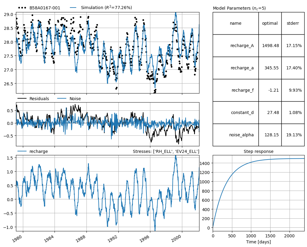
Finally we can extract a single model from the pastastore to visualise its results.

[20]:

# results from a single model
ml1 = pstore.get_models("B58A0167-001")
ml1.plots.results()

[20]:

[<Axes: ylabel='Head'>,
 <Axes: >,
 <Axes: title={'right': "Stresses: ['RH_ELL_377', 'EV24_ELL_377']"}, ylabel='Rise'>,
 <Axes: title={'center': 'Step response'}>,
 <Axes: title={'left': 'Model parameters ($n_c$=4)'}>]

../_images/examples_03_hydropandas_and_pastas_39_1.png

Hydropandas and Pastas

Groundwater observations

Meteo observations

Pastas model

Surface water observations

Pastastore

Groundwater observations

Meteo

Creating and solving models

Groundwater observations 

Meteo observations 

Pastas model 

Surface water observations 

Pastastore 