Exploring groundwater data from Lizard
In this notebook, you will experiment how to use the hydropandas package to access, visualize and explore meta data from Lizard, a cloud datawarehouse that can be used to store groundwater observations. Data sources:
Vitens (default, public access): Vitens is the largest drinking water company in the Netherlands, and it has more than 10.000 groundwater wells and more than 50.000 timeseries in its datawarehouse. The data spans from the 1930’s to the present, and it is constantly updated with new observations. Vitens also validates the data using ArtDiver and provides quality flags and comments for each observation. The data is open to the public and you can find more information at https://vitens.lizard.net.
Others: If you have access to other Lizard data sources, you can specify the
organisationparameter in thelizardfunctions to access those data sources. Currently, only “vitens” is officially supported. Note that you then may need to specify authentication as well by means of a personal API key. This has been implemented for the municipality of Rotterdam.
Feel free to customize and expand upon this introduction as needed.
Notebook contents
Read groundwater timeseries
Analyse groundwater observations
Build a Pastas model
[1]:
import pastas as ps

import hydropandas as hpd
[2]:
hpd.util.get_color_logger("INFO")
[2]:
<RootLogger root (INFO)>
1. Read groundwater timeseries
1.1 Authentication
The vitens data source is used by default, and does not require authentication. If you have access to other Lizard data sources, you can specify the organisation parameter in the read_lizard function to access those data sources. Currently, only “vitens” is officially supported.
For others than Vitens, you may need authentication. You can use the auth parameter to pass your credentials. According to the Lizard documentation, you should create a personal API key at https://{organisation}.lizard.net/management/ and enter that in the cell below. If you do not have access to other data sources, you can use auth=None to skip authentication.
[3]:
## Lizard uses the organisation parameter to specify the data source.
organisation = "vitens"  # or: "rotterdam"
auth = None

## UNCOMMENT AND SET YOUR API KEY IF YOU NEED TO SPECIFY CREDENTIALS
# your_api_key = "your_api_key_here"
# auth = ("__key__", your_api_key)
Which timeseries to include? (which_timeseries)
In the Lizard database, the follow WNS codes are used:
WNS9040.hand: Hand measurements (in Hydropandas: “hand”)
WNS9040: Diver measurements (in Hydropandas: “diver”)
WNS9040.val: Validated diver measurements (in Hydropandas: “diver_validated”)
Use of WNS codes per organisation:
Vitens uses only categories 1 and 2. So for consistency with previous versions, Hydropandas will use “hand” and “diver” measurements when
which_timeseriesis not specified.Rotterdam uses all three categories. So for Rotterdam you can use
which_timeseries=["hand", "diver", "diver_validated"]to get both the validated and unvalidated diver measurements.
1.1 Get observations from extent
Use read_lizard to find monitoring wells by specifying a geographical extent in Rijksdriehoeks coordinates.
[4]:
my_extent = (137_000, 138_000, 458_000, 459_000)
oc = hpd.read_lizard(
    extent=my_extent,
    which_timeseries=["hand", "diver", "diver_validated"],
    datafilters=None,
    combine_method="merge",
    organisation=organisation,
    auth=auth,
)
INFO:hydropandas.io.lizard.get_obs_list_from_extent:Number of monitoring wells: 1
INFO:hydropandas.io.lizard.get_obs_list_from_extent:Number of pages: 1
Page: 100%|██████████| 1/1 [00:00<00:00,  2.08it/s]
monitoring well:   0%|          | 0/1 [00:00<?, ?it/s]
INFO:hydropandas.io.lizard.get_timeseries_uuid:Successfully retrieved 848 timeseries events for UUID cd5bb67c-4b74-4c8a-8a59-511d2e89a333
INFO:hydropandas.io.lizard.get_timeseries_uuid:Successfully retrieved 34993 timeseries events for UUID 51219e93-8fc7-4bdd-8d1b-bbbd6ef4b18b
INFO:hydropandas.io.lizard.get_timeseries_uuid:Successfully retrieved 679 timeseries events for UUID d9441bc1-8909-48b6-bf5f-94706535a321
INFO:hydropandas.io.lizard.get_timeseries_uuid:Successfully retrieved 679 timeseries events for UUID 55e5394d-41f2-48d8-b139-a24887b9e370
monitoring well: 100%|██████████| 1/1 [00:08<00:00, 8.04s/it]
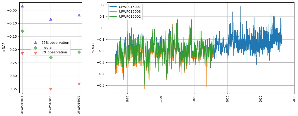
Visualize all groundwater wells inside the extent on a map (visualize the ObsCollection). The markers are clickable to show a preview of the availables observations.
[5]:
oc.plots.interactive_map(
    color="red", zoom_start=15, tiles="Esri.WorldImagery", popup_width=350
)
[5]:
Print all the retrieved groundwater wells and tubes, and make a plot of the observations.
[6]:
oc
[6]:
| x | y | location | filename | source | unit | tube_nr | screen_top | screen_bottom | ground_level | tube_top | metadata_available | obs | lat | lon | |
|---|---|---|---|---|---|---|---|---|---|---|---|---|---|---|---|
| name | |||||||||||||||
| UPWP016001 | 137401.64297 | 458893.683528 | B31H0580 | lizard | m NAP | 1 | -22.43 | -24.43 | 1.58 | 2.198 | True | GroundwaterObs UPWP016001 -----metadata------ ... | 52.117985 | 5.13026 | |
| UPWP016003 | 137401.64297 | 458893.683528 | B31H0580 | lizard | m NAP | 3 | -65.43 | -67.43 | 1.58 | 2.141 | True | GroundwaterObs UPWP016003 -----metadata------ ... | 52.117985 | 5.13026 | |
| UPWP016002 | 137401.64297 | 458893.683528 | B31H0580 | lizard | m NAP | 2 | -53.93 | -55.93 | 1.58 | 2.178 | True | GroundwaterObs UPWP016002 -----metadata------ ... | 52.117985 | 5.13026 |
[7]:
oc.obs.values[0]
[7]:
hydropandas.GroundwaterObs
| UPWP016001 | |
|---|---|
| x | 137401.64297 |
| y | 458893.683528 |
| location | B31H0580 |
| filename | |
| source | lizard |
| unit | m NAP |
| tube_nr | 1 |
| screen_top | -22.43 |
| screen_bottom | -24.43 |
| ground_level | 1.58 |
| tube_top | 2.198 |
| metadata_available | True |
| value | flag | comment | origin | |
|---|---|---|---|---|
| peil_datum_tijd | ||||
| 1976-04-15 12:00:00 | -0.300 | 0 | hand | |
| 1976-04-28 12:00:00 | -0.260 | 0 | hand | |
| 1976-05-18 12:00:00 | -0.330 | 0 | hand | |
| 1976-06-02 12:00:00 | -0.230 | 0 | hand | |
| 1976-06-17 12:00:00 | -0.300 | 0 | hand | |
| ... | ... | ... | ... | ... |
| 2026-03-30 03:00:00 | -0.093 | 0 | diver | |
| 2026-03-30 06:00:00 | -0.088 | 0 | diver | |
| 2026-03-30 09:00:00 | -0.094 | 0 | diver | |
| 2026-03-30 12:00:00 | -0.104 | 0 | diver | |
| 2026-03-30 12:26:35 | -0.122 | 0 | hand |
35841 rows × 4 columns
[8]:
oc.plots.section_plot(plot_obs=True)
INFO:hydropandas.extensions.plots.section_plot:created sectionplot -> UPWP016001
INFO:hydropandas.extensions.plots.section_plot:created sectionplot -> UPWP016003
INFO:hydropandas.extensions.plots.section_plot:created sectionplot -> UPWP016002
[8]:
(<Figure size 1500x500 with 2 Axes>,
 [<Axes: ylabel='m NAP'>, <Axes: ylabel='m NAP'>])
2. Analyse Groundwater observations
Now lets download the groundwater level observation using the from_lizard function of a GroundwaterObs object. The code below reads the groundwater level timeseries for the well UPWP016 from Lizard and makes a plot.
[9]:
gw_lizard = hpd.GroundwaterObs.from_lizard(
    "UPWP016",
    tmin="1900-01-01",
    tmax="2030-01-01",
    organisation="vitens",
    auth=auth,
)
print(gw_lizard)

ax = gw_lizard["value"].plot(
    figsize=(12, 5),
    marker=".",
    grid=True,
    label=gw_lizard.name,
    legend=True,
    xlabel="Date",
    ylabel="m NAP",
    title="Groundwater observations for " + gw_lizard.name,
)
INFO:hydropandas.io.lizard.get_timeseries_uuid:Successfully retrieved 848 timeseries events for UUID cd5bb67c-4b74-4c8a-8a59-511d2e89a333
INFO:hydropandas.io.lizard.get_timeseries_uuid:Successfully retrieved 34993 timeseries events for UUID 51219e93-8fc7-4bdd-8d1b-bbbd6ef4b18b
GroundwaterObs UPWP016001
-----metadata------
name : UPWP016001
x : 137401.64297031244
y : 458893.6835282739
location : B31H0580
filename :
source : lizard
unit : m NAP
tube_nr : 1
screen_top : -22.43
screen_bottom : -24.43
ground_level : 1.58
tube_top : 2.198
metadata_available : True

-----time series------
                     value  flag comment origin
peil_datum_tijd
1976-04-15 12:00:00 -0.300     0           hand
1976-04-28 12:00:00 -0.260     0           hand
1976-05-18 12:00:00 -0.330     0           hand
1976-06-02 12:00:00 -0.230     0           hand
1976-06-17 12:00:00 -0.300     0           hand
...                    ...   ...     ...    ...
2026-03-30 03:00:00 -0.093     0          diver
2026-03-30 06:00:00 -0.088     0          diver
2026-03-30 09:00:00 -0.094     0          diver
2026-03-30 12:00:00 -0.104     0          diver
2026-03-30 12:26:35 -0.122     0           hand

[35841 rows x 4 columns]
The groundwater observations contain a validation flag per timestamp. These can ‘betrouwbaar’ (reliable), ‘onbetrouwbaar’ (unreliable) en ‘onbeslist’ (unvalidated). Below flags of the timeseries are shown as a percentage, and the unreliable timestamps are printed.
[10]:
print(gw_lizard["flag"].value_counts(normalize=True) * 100)
gw_lizard[gw_lizard["flag"] == "onbetrouwbaar"]
flag
0    99.960939
1     0.016741
7     0.013951
6     0.005580
3     0.002790
Name: proportion, dtype: float64
[10]:
hydropandas.GroundwaterObs
| UPWP016001 | |
|---|---|
| x | 137401.64297 |
| y | 458893.683528 |
| location | B31H0580 |
| filename | |
| source | lizard |
| unit | m NAP |
| tube_nr | 1 |
| screen_top | -22.43 |
| screen_bottom | -24.43 |
| ground_level | 1.58 |
| tube_top | 2.198 |
| metadata_available | True |
| value | flag | comment | origin | |
|---|---|---|---|---|
| peil_datum_tijd |
3. Create a Pastas model
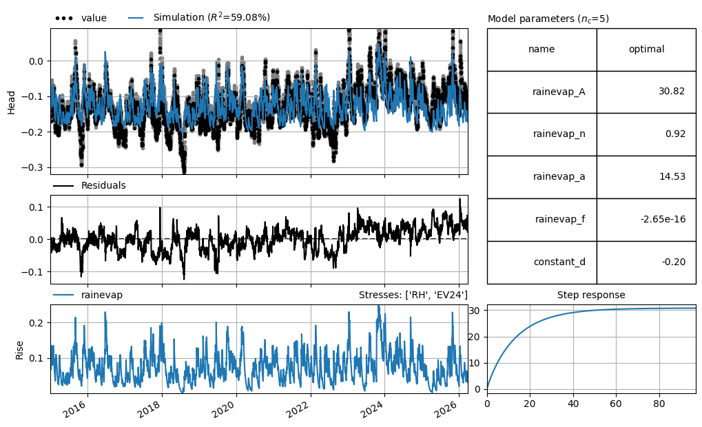
Lets make a Pastas model for this groundwater well (starting from 2015) and use the nearest KNMI station for meteorological data
[11]:
# Get the precipitation and evaporation data from the KNMI
precipitation = hpd.PrecipitationObs.from_knmi(
    xy=(gw_lizard.x, gw_lizard.y),
    start=gw_lizard.index[0],
    end=gw_lizard.index[-1],
    fill_missing_obs=True,
)
evaporation = hpd.EvaporationObs.from_knmi(
    xy=(gw_lizard.x, gw_lizard.y),
    meteo_var="EV24",
    start=gw_lizard.index[0],
    end=gw_lizard.index[-1],
    fill_missing_obs=True,
)

# Create a Pastas Model
ml = ps.Model(
    gw_lizard.loc[gw_lizard["origin"] == "diver", "value"], name=gw_lizard.name
)

# Add the recharge data as explanatory variable
ts1 = ps.RechargeModel(
    precipitation["RH"].resample("D").first(),
    evaporation["EV24"].resample("D").first(),
    ps.Gamma(),
    name="rainevap",
    settings=("prec", "evap"),
)

# Add the stressmodel to the model and solve for period after 2015
ml.add_stressmodel(ts1)
ml.solve(tmin="2015")
ml.plots.results(figsize=(10, 6))
INFO:hydropandas.io.knmi.get_knmi_obs:get KNMI data from station nearest to coordinates (137401.64297031244, 458893.6835282739) and meteovariable RH
INFO:hydropandas.io.knmi.fill_missing_measurements:knmi station De Bilt has no measurements for RH after 2026-03-30 01:00:00 and an end date of 2026-03-30 12:26:35 was requested. Changing end to 2026-03-30 01:00:00
INFO:hydropandas.io.knmi._add_missing_indices:station 260 has no measurements after 2026-03-30 01:00:00
INFO:hydropandas.io.knmi.get_knmi_obs:get KNMI data from station nearest to coordinates (137401.64297031244, 458893.6835282739) and meteovariable EV24
INFO:hydropandas.io.knmi.fill_missing_measurements:knmi station De Bilt has no measurements for EV24 after 2026-03-30 01:00:00 and an end date of 2026-03-30 12:26:35 was requested. Changing end to 2026-03-30 01:00:00
INFO:hydropandas.io.knmi._add_missing_indices:station 260 has no measurements after 2026-03-30 01:00:00
WARNING:pastas.timeseries._validate_series:The Time Series 'value' has nan-values. Pastas will use the fill_nan settings to fill up the nan-values.
INFO:pastas.timeseries._fill_nan:Time Series 'value': 12 nan-value(s) was/were found and filled with: drop.
INFO:pastas.timeseries._fill_after:Time Series 'RH' was extended in the future to 2026-03-30 00:00:00 with the mean value (0.0024) of the time series.
INFO:pastas.timeseries._fill_after:Time Series 'EV24' was extended in the future to 2026-03-30 00:00:00 with the mean value (0.0017) of the time series.
Fit report UPWP016001                Fit Statistics
===================================================
nfev     12                     EVP           59.08
nobs     4107                   R2             0.59
noise    False                  RMSE           0.03
tmin     2015-01-01 00:00:00    AICc      -27654.96
tmax     2026-03-30 12:00:00    BIC       -27623.37
freq     D                      Obj            2.44
freq_obs None                   ___
warmup   3650 days 00:00:00     Interp.          No
solver   LeastSquares           weights          No

Parameters (5 optimized)
===================================================
                 optimal     initial  vary
rainevap_A  3.082213e+01  198.385164  True
rainevap_n  9.241377e-01    1.000000  True
rainevap_a  1.453124e+01   10.000000  True
rainevap_f -2.651398e-16   -1.000000  True
constant_d -2.041333e-01   -0.126311  True

Warnings! (1)
===================================================
Parameter 'rainevap_f' on upper bound: 0.00e+00
[11]:
[<Axes: xlabel='peil_datum_tijd', ylabel='Head'>,
 <Axes: >,
 <Axes: title={'right': "Stresses: ['RH', 'EV24']"}, ylabel='Rise'>,
 <Axes: title={'center': 'Step response'}>,
 <Axes: title={'left': 'Model parameters ($n_c$=5)'}>]